


PaleoScan™ coloured inversion: Show your true colours
Inversion of seismic data to acoustic impedance often requires time and expertise. To overcome this, Coloured Inversion (Lancaster and Whitcombe, 2000) is a quick technique which can be easily applied on seismic data and performs a simple understandable inversion process. It is designed to match approximately the average spectrum of the inverted seismic data with the observed impedance. Thanks to the interactive and real time capabilities of PaleoScan™, the optimum operator can be quickly estimated from acoustic impedance logs and seismic amplitudes. Moreover, by inserting an a priori model as an input constraint, absolute values can be computed.
Drag and drop the seismic volume and some acoustic impedance logs, let’s colour that data !
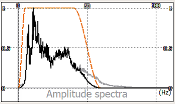
1. Estimating the seismic amplitude spectrum
Knowing the frequency content of the seismic data before starting the process is essential. The bounding box allows the user to focus on the area of interest in order to estimate the average amplitude spectrum. Thus undesired seismic traces will be excluded. The aim is then to increase the low frequency content and reduce the high frequencies (in contrast to the Spectral Blueing workflow). The orange curve is the Hann band pass filter which is applied to seismic spectrum –original in grey, filtered in black.
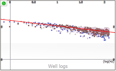
2. Linear trending the logs spectra
Theoretically, the well amplitude spectrum is similar to the function f^β, with f the frequency and β a positive constant (Lancaster and Whitcombe, 2000). Indeed, the Earth’s reflectivity favours high frequencies, with some frequencies having more energy (hence coloured inversion – in contrast to a white spectrum). The acoustic impedance spectra have the same behaviour but with a negative constant α. These are displayed in a log/log scale to estimate the constant value, which corresponds to the slope of the regression. α should vary between -0.8 and -0.6.
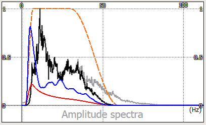
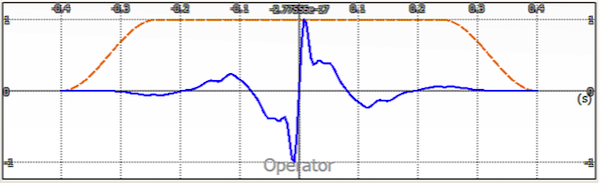
3. Looking at the operator spectrum
The operator amplitude spectrum (shown in blue) is then computed from the seismic (black) and the wells (red) amplitudes spectra. The low frequencies should be increased and the high ones attenuated. If not, previous parameters for filtering can be adjusted in real time.
4. Shaping the operator
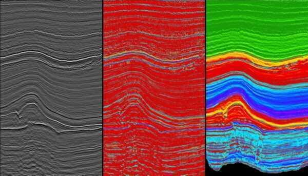
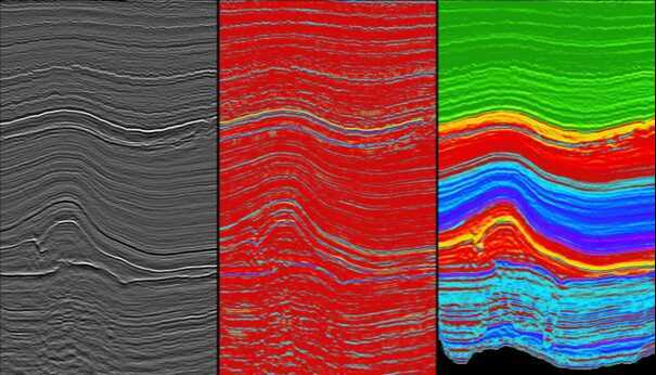
5. Interpreting the results
The final operator is then convolved with the input volume and a preview is displayed. The preview is updated in real time for all parameters. The operator can be saved as a wavelet, and then be convolved with another volume at a later stage. The final output is then a relative acoustic impedance volume, similar to a band-limited inversion result but quickly computed.
6. Going further
To get absolute values, a low-frequency model can be added to the relative output. In PaleoScan™, this a priori model is easily computed from the Properties Modeling add-on which propagates the logs into the relative geological time model.
Coloured Inversion in PaleoScan™ is a fast way to preview and compute a seismic inversion result. It allows the enhancement of seismic resolution, features, discontinuities and your seismic interpretation process.
To learn more about PaleoScan™ and the Coloured Inversion tool, drop us a line at contact@eliis.fr.
References
Lancaster, S., and D. Whitcombe, 2000, Fast-track ‘coloured’ inversion. SEG Expanded Abstracts, 1572–1575.