


Questions and Answers
Installation & Settings
Unfortunately, we don’t have a silent installer available from our website. But here is another way to install PaleoScan silently on your machines, from the command prompt:
Use the following syntax: paleoscan.exe /S /D=C:\destination_folder
You may want to use the same arguments for the uninstall executable: uninstall.exe /S
Let us know if this helps.
The version of the Petrel Data Connector that you should use depends on both your version of Petrel and your version of Paleoscan. For example, if you are using Paleoscan 2023.x.x and Petrel 2022 you should use the "PaleoScan 2023-Petrel 2022" version of the connector.
You can find the different versions of the PaleoScan connectors just here https://www.eliis-geo.com/connect-a.html
For each version of Paleoscan, we officially support connectors for the versions of Petrel of the same year and for the previous year's Petrel version. Exceptionally, we may release connectors for older versions of Petrel.
Unsupported versions of the connector (e.g. when the Petrel version is more recent than the Paleoscan version, or when there is more than two years difference between both versions) may work and facilitate the transfer of data between Petrel and Paleoscan, however, we do not guarantee the integrity of the transfer in such scenarios. When attempting to use a connector in an unsupported scenario, you should always take Petrel's version as reference.
For example:
• If you work with PaleoScan 2021 and Petrel 2019, the Data Connector you should use is "Petrel 2019 ← → PaleoScan 2020"
• If you work with PaleoScan 2019 and Petrel 2021, the Data Connector you should use is "Petrel 2021 ← → PaleoScan 2021"
PaleoScan runs on PCs, laptop, desktop or workstation. PaleoScan does not run on Mac computers. PaleoScan can also run on Virtual Machines.
PaleoScan requires Windows 64-bit version 7 or above.
The minimum /recommended hardware configuration to run PaleoScan is:
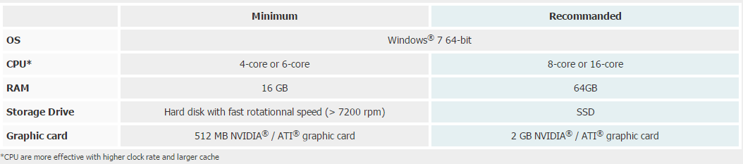
The recommendation for the percentage of physical memory allocated to PaleoScan is to keep the 30% default value for a machine with at least 16GB of RAM.
The “Temporary Directory” stores intermediate volumes computed by PaleoScan. The “Temporary Directory” does not need to be at the same location than the PaleoScan project and can be set by the user. It must however have at least 3 times the size of the seismic volume of free space.
The recommendation for GPU usage is to select the graphic card and for the CPU usage is to keep the default number of threads. Note that enabling the GPU parallelization will not dramatically increase Paleoscan’s performance except for the Properties Modeling module.
CPU parallelization is widely used in PaleoScan but GPU acceleration (using OpenCL technology) is currently used only in the Properties Modeling module and for some attributes computation, such as similarity. When both are enabled, GPU is used instead of CPU for the processes that support GPU. The other processes that do not support GPU but CPU parallelization run faster when CPU multithreading (several threads running on the same CPU) is enabled. However, all the threads are processed on the machine running PaleoScan and share the machine’s memory. Threads cannot be processed separately on different CPUs and memories. Paleoscan’s tasks (Geo-Model, attributes computation...) can only be started from the PaleoScan GUI (Graphical User Interface) as single executables. Distributed environments, with several physical machines with separated memory and CPU, are therefore not supported.
Our internal benchmarks show that PaleoScan’s performance does not increase linearly with the number of cores used: 8 cores will definitely improve the performance but it will peak at 16 cores and even decrease beyond 16.
PaleoScan accesses hard drives intensely for reading from and writing to the flat file database. PaleoScan therefore works best when Input/Output to hard drives is optimized, either by working locally or through a network with the application and the memory disks at the same physical location. Using Solid State Drives with increased I/O speed will also improve performance.
PaleoScan can import 8/16 bit Segy data and then keeps the original data size. However, almost all the steps of the PaleoScan workflow will create 32 bit volumes (attribute computation, Model-Grid...). As a result, the output volume size is bigger (x2 if 16 bits, x4 if 8 bits) than the original volume.
It is probably a graphic card issue. The user needs to check in the computer settings that the right graphic card is assigned to PaleoScan.
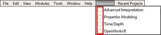
The add-on module needs to be activated through an extension available with a specific license.
Go to the Extensions menu and click on the add-on module(s) to activate them.
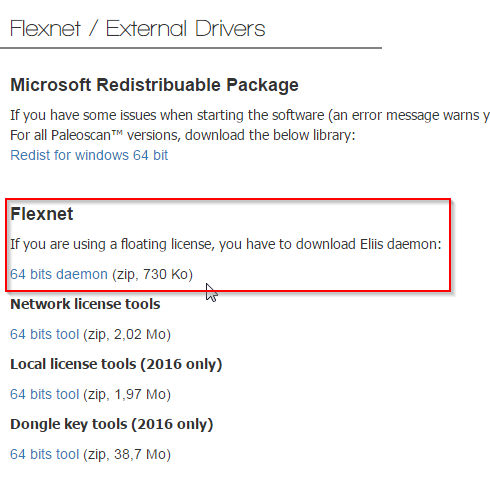
The latest PaleoScan uses an updated FlexNet License system. This implies that the license server needs to be updated, the Eliis daemon can be found on our Download page.
In the installation folder of PaleoScan 2018, for example: "C:\Program Files\Eliis\PaleoScan\2018.1\licensing\eliis.exe"
On our website (you need a login and password to access our extranet): Download
Got a question ?
We'll be thrilled to hear from you !
Customer support
Data loading/Exporting
To reduce the loading time, one advice is to upload your SEGY exactly where PaleoScan is installed on your computer (not next to your project, but next to your PaleoScan launcher) However, if you consider that it is still too long, you can try to import something smaller.
To avoid importing heavy seismic which would take time to load and take space, you have three options available during the importation process.
First, you can decimate your volume.
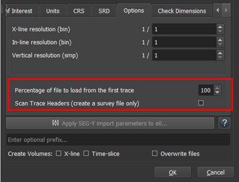
In the "Options" tab, you can change the bin/sample size.
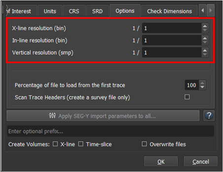
For instance, with a set up at 1/2, it means that PaleoScan™ will load one line out of two for each direction (Inline, Xline and Time Slice).
Depending on the resolution of your SEGY, you could apply for instance the following:
X-line resolution: 1/2
In-Line resolution: 1/2
For example, if your seismic has a bin size of 12.5 m, you will get a resolution of 25 m.
Moreover, another option can be useful to test your importation: Percentage of the file to import. By default, all the seismic is imported, you can choose to import only a lower percentage.
The Scan Trace Header option aims at only importing the survey without the seismic traces (very useful to know the seismic size!).
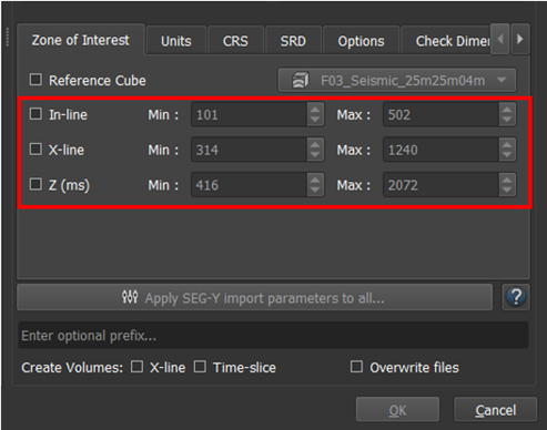
Secondly, you can crop your seismic defining the Min and Max values in every direction. These options are available from the “Zone of interest” tab.
A volume encoded in 8 bytes imported manually in PaleoScan, will be created/read in 8 bytes, and therefore the size of the volume will not change. However as soon as an object is created (grid, etc) from this volume, the new volume/object will be encoded in 32 bytes and so the size will be multiplied by 4.
By importing a volume from Petrel into PaleoScan with the plug-in, a volume of 8 bytes will be directly converted into 32 bytes in PaleoScan, and so the size of the volume will be multiplied by 4.
Approximations are made during this transfer via the Petrel connector, so it is normal to have a volume of a little different size than expected (for example: volume in 8 bytes of 24 GB in Petrel, should arrive in 32 bytes in PaleoScan with a size of 96 GB, but may have instead a size of 88.9 GB).
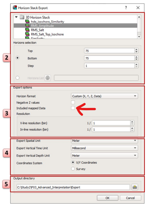
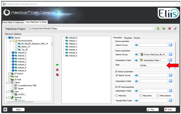
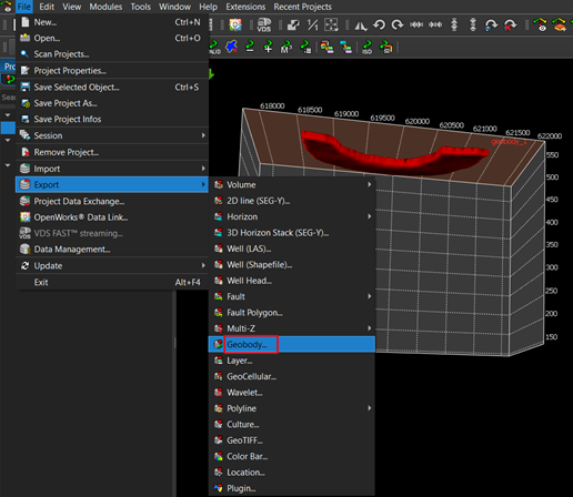
There are a couple of ways we could do this. You could Export the horizons from the Horizon Stack with X, Y, Z, and Data (Option 1), and you could extract each surface as individual horizons in your project and then transfer them to Petrel with the connector (Option 2).
Option 1:
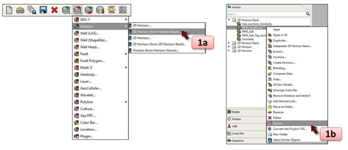
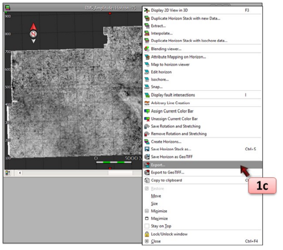
You can export the horizons from the Horizon Stack.
The option is available from:
1a- The general toolbar,
1b- The context menu of the horizon stack in the Project Browser
1c- The horizon stack viewer.
Here are the step-by-step in Petrel, which can be implemented theoretically in the software you are using:
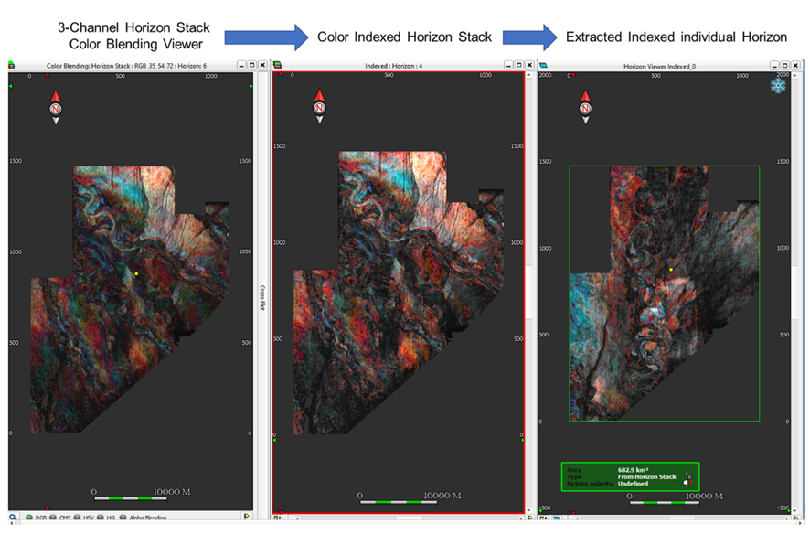
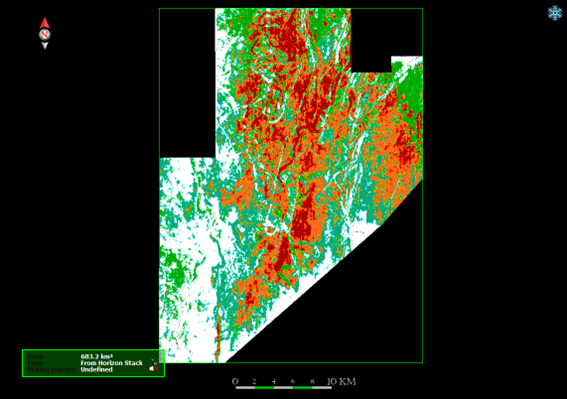
Before we start with the workflow, please remember you will first need to have the horizons from the 3-Channel Horizon Stack Color Blending Viewer saved as a Color Indexed Horizon Stack (if you don’t know how to do it, please see the step-by-step at the end of the message*), from which you can create/extract the Color Indexed individual horizons (these are the only ones you can transfer back to Petrel for example, not Horizon Stacks).
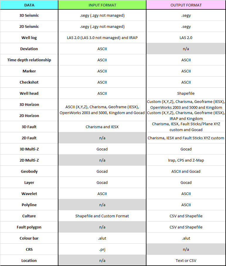
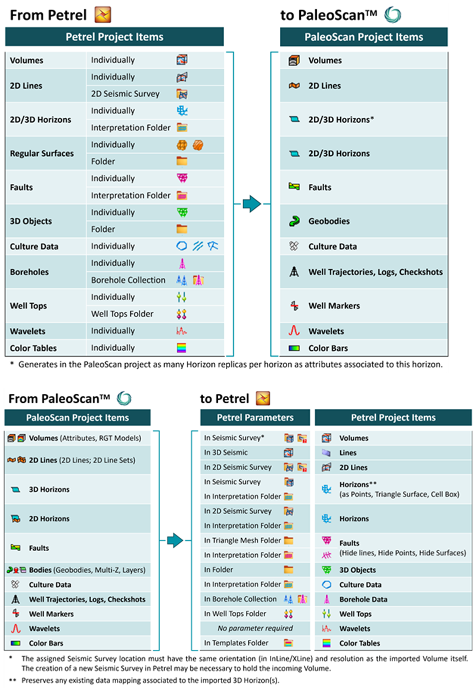
Eliis has developed two data connectors: Petrel® and OpenWorks®.
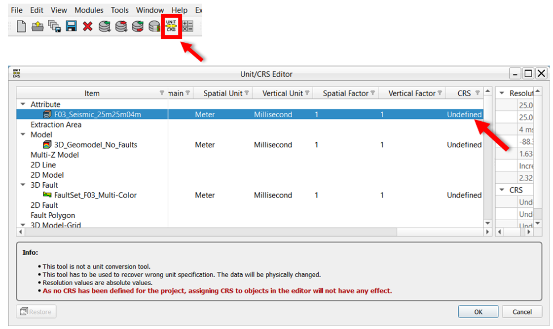
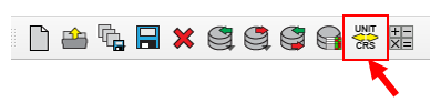
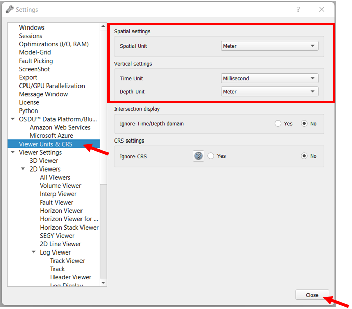
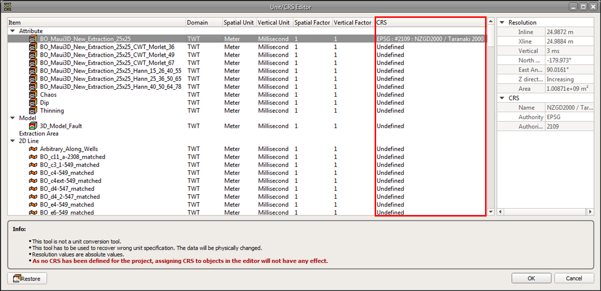
It is possible to change the unit of certain objects by clicking on the UNIT/CRS Editor icon. This tool is a correction tool and not a conversion tool, it changes the unit of the objects.
Platform
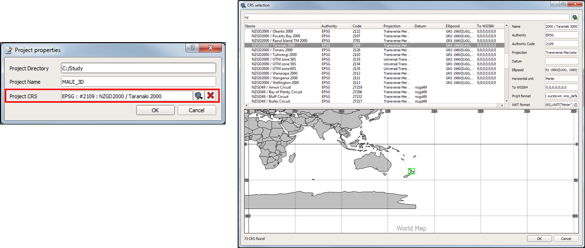
The best way to add a new CRS into PaleoScan when you are in possession of the prj file consists in importing it (see image below). Importation prevents any parsing issue due to inaccuracy entering the CRS manually as a proj4, wkt format or via the form (also note that PaleoScan only manages UTM coordinate CRS; Geographic coordinate CRS are not managed).
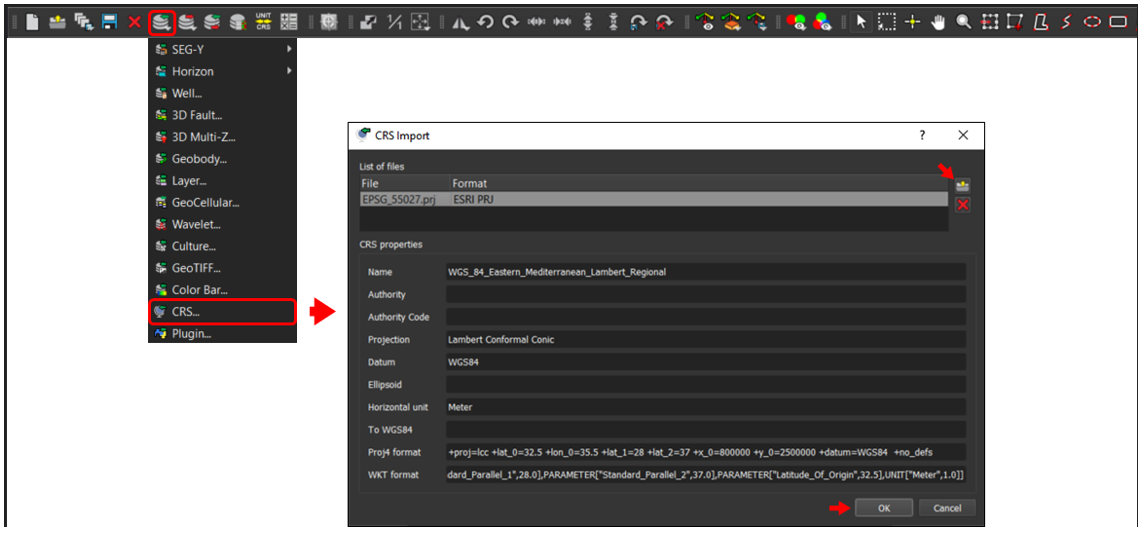
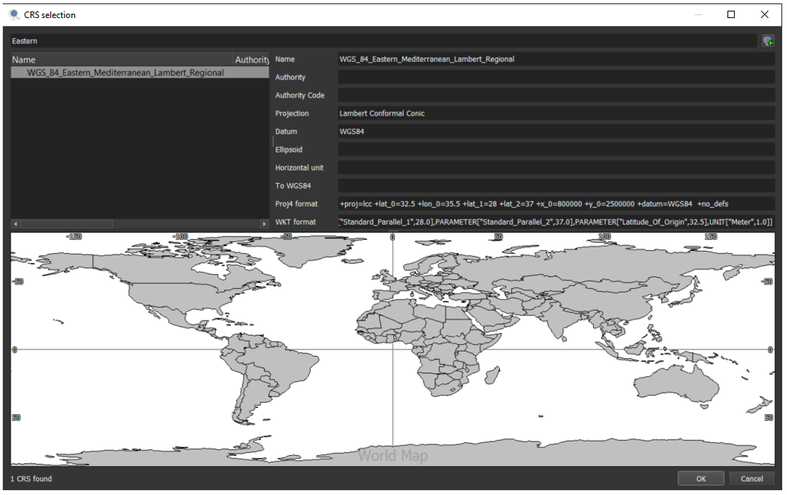
This way, the imported CRS will appear in your Project Browser (in the "Other" tab) and will be listed in the CRS menus next time you want to assign it to the project or to individual objects (note that, unlike pre-existing CRS; the green localization framing of an imported CRS may not appear in the world projected map).
There's no need to start a project from scratch. You can change the project's CRS at any time at File/Project Properties...
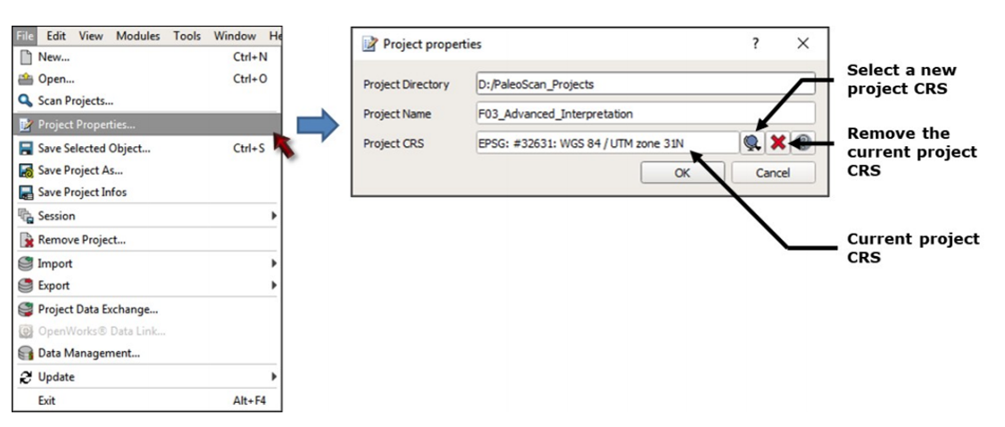
Also, if you need to change the CRS of an object in your project, access the Unit/CRS editor. Drag the slider on the right, double click on the CRS column and change/define a CRS.
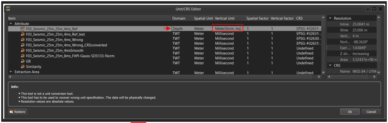
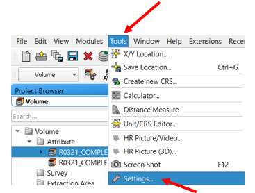
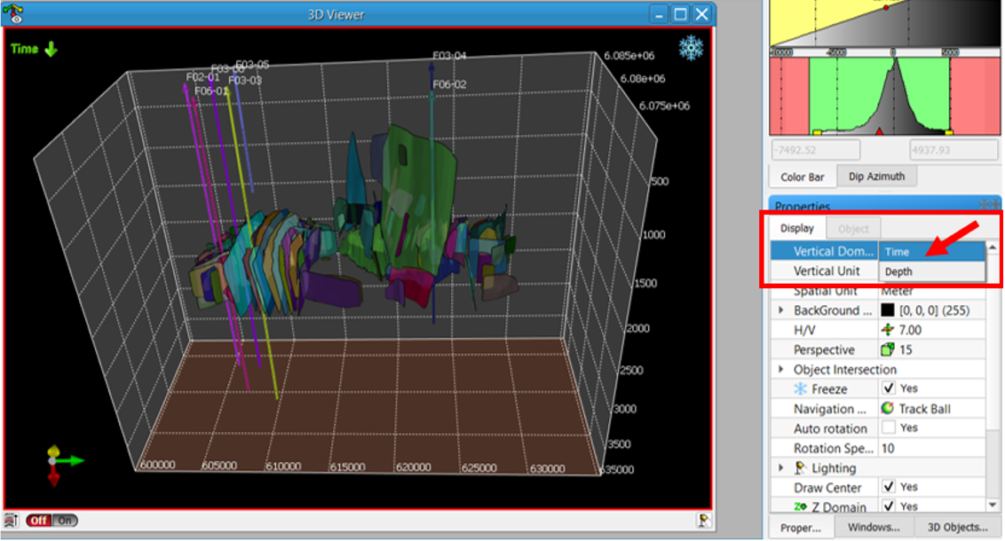
You can change the vertical dimension of your seismic volume directly in PaleoScan:
From the Main toolbar, go in the Unit/CRS Editor. Then in the displayed interface, change the Vertical Unit to the desired unit (see image below) (the Domain should change automatically accordingly). Eventually, click OK at the bottom right of the interface to apply the change.

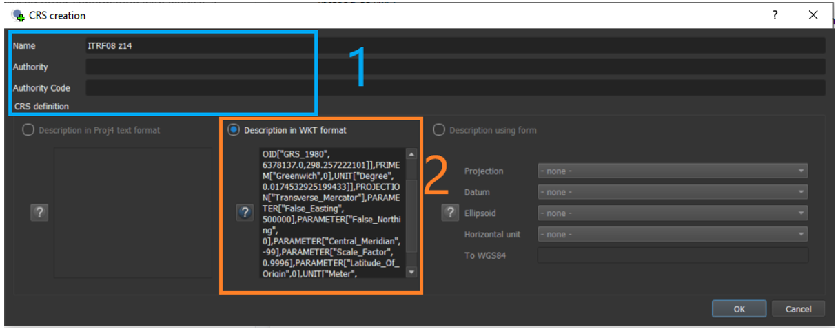
It is possible to create a custom CRS in PaleoScan if those CRS are not as default in the current list. The CRS creation interface can be reached from the CRS selection window or from the Tools menu:
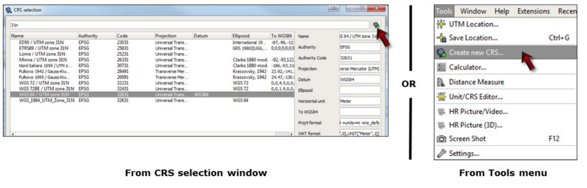
From there, fill the CRS creation form:
1. The first three parameters (name, authority, and authority code) are information parameters.
2. The CRS definition can be filled in 3 ways:
• Using the proj4 format, which is the native CRS format used by PaleoScan. It is the recommended way to define a custom CRS. An exhaustive list of proj4 definition parameters can be found here: https://proj.org/usage/projections.html
• Using the WKT (Well Known Text) format. The WKT definition will be converted in proj4 format by PaleoScan. If a proj4 definition is available, prefer to use it instead of WKT.
• Using a dedicated form. This method is not exhaustive, but it can be used for simple CRS definitions.
In this case, I would recommend using the WKT which was accepted by PaleoScan. You could copy and paste everything from the shared txt files into the WKT field:
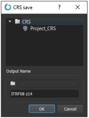
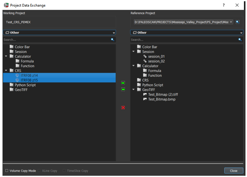
Since the customized CRS will be available in the Project Browser, you could then transfer the saved CRS between projects using the Project Data Exchange between projects.
Question:
"I have a question about mixing CRS with different datums – is there any coordinate operation (transformation) undertaken by PaleoScan if a horizon is pushed back to Petrel with a different CRS to that of the project, or are you leaving all of this to the Petrel projection engine? Essentially, is the assignment of CRS to objects in PaleoScan purely on a “metadata” level, or are there actual geodetic calculations being undertaken in the software?"
Answer:
1. When exporting to Paleoscan
For seismic cubes, 3D-Lines. We apply a transform on the cube location using Petrel Engine in order to express its coordinates in the chosen CRS option(object or project). The cube data itself, is expressed using the indices of the cube so it does not require geospatial conversions.
For 3D-Horizons and surfaces,
in addition to the bounding box location, we also convert the data (3D points) using a transform provided by petrel engine in order to express the data in the chosen CRS option(object or project).
For other objects,
coordinates are expressed in Project CRS regardless of the chosen CRS option, the CRS is considered as purely "metadata".
2. When importing back in Petrel
For all objects, we assign the CRS as purely "metadata".
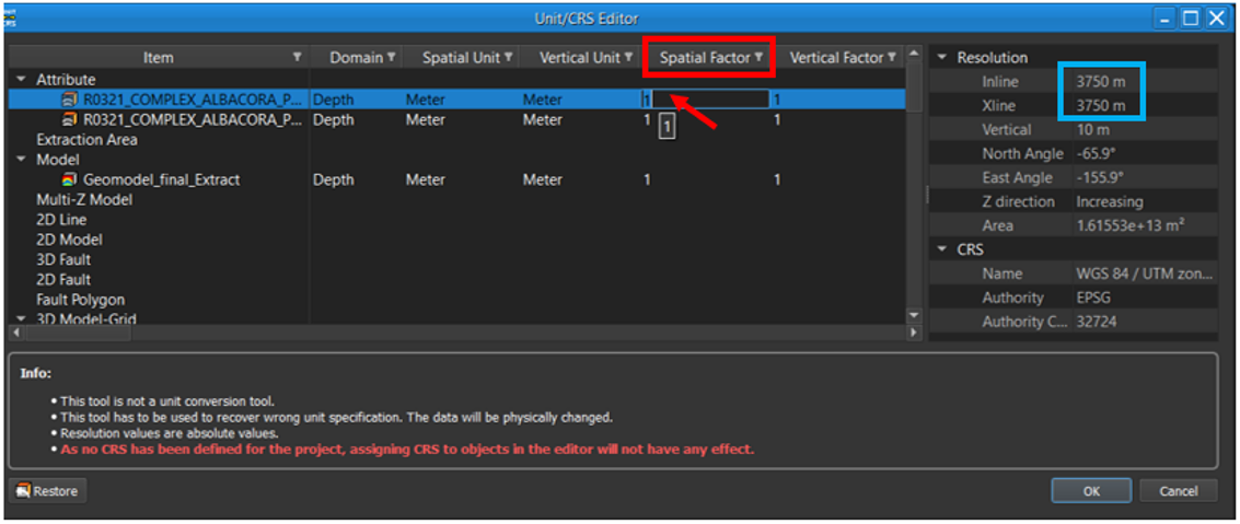
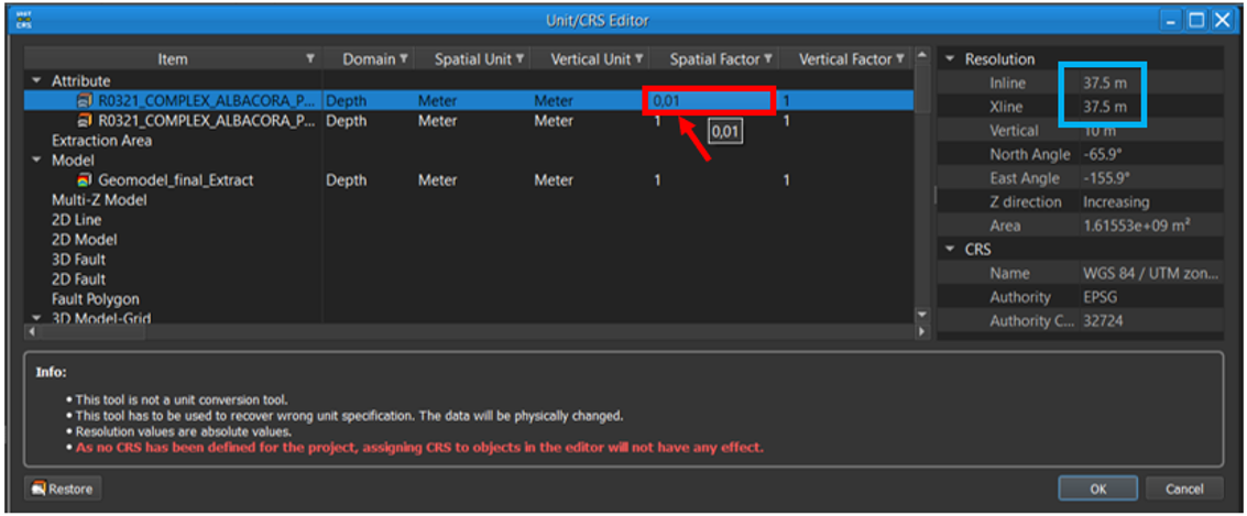
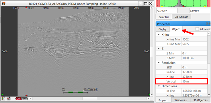
You can easily fix your seismic resolution if it has a wrong spatial or vertical factor (for example: In-line resolution 3750m instead of 37.5m).
From the Main toolbar, go in the Unit/CRS Editor.
Then select the object, double-click on Spatial Factor (or Vertical Factor) and change it. In our example, the Inline and Xline resolution is 3750 m (you can check this information on the right side of the window). Thus, we will change the Spatial factor to 0.01. The resolution is automatically updated on the right.
Finally, a window pops up resuming the unit changes that will be applied. Click on Ok to confirm.
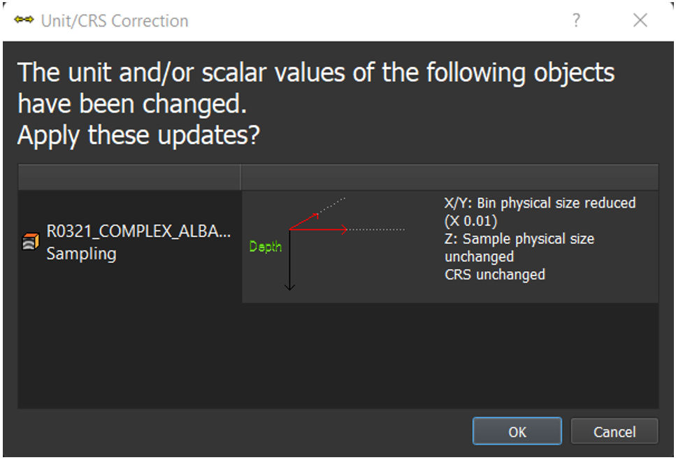
Note that if you had already computed objects from this seismic volume, you would have to apply them this factor as well.
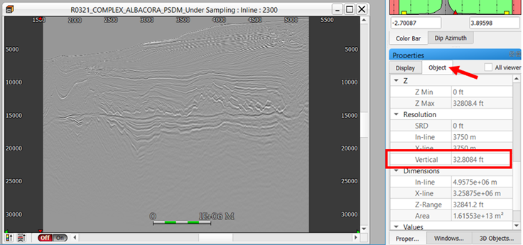
When you import an object, you have to define the spatial and vertical units. For instance, if you import a volume in depth, that is in meter, and you define the correct units at the importation step. You could still have wrong units displayed because the viewers are set with other units than the imported object.
You can check the unit of your viewer from the Properties, on the Object tab. Go down until you find the information about the resolution.
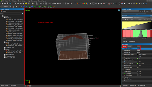
If you are struggling with the 3D viewer to display some objects, it is probably due to the vertical domain of the 3D viewer. Fortunately, it is easy to change the domain.
1- Use the selection mouse mode by pressing F
2- Select the 3D viewer, you have to doble click on it. It appears with red edges.
3- From the properties, check if the domain is the correct one.
PaleoScan can deal with different types of units (foot, meter, mile, yard, inch). For the wells, all the data are converted in meters into the application.
The CRS of a project can be defined upon creation and can be modified later on.
The CRS of each object (seismic volumes, horizons, wells…) can be specified upon import and can be modified later on in the Unit/CRS Editor.
When PaleoScan™ creates volumes, they are first generated as temporary file. If there is a lack of disk space, the user can change the location of the temp. file via “Tools/Settings/Optimizations”.


The cursor can be displayed simultaneously all viewers by activating the cursor option from the Properties window of each viewer.

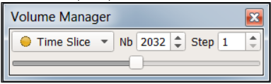
By default, PaleoScan™ always generates/displays the Inline. To generate/display the Crossline/Time Slice, the user has to open a volume, then from the Volume Manager widget, click on the Inline tab and then click on Xline or Time Slice.

To synchronize colour bars, the user has to click on the viewer which has the colour bar he wants to use, then keep holding down the ALT keyboard and drag and drop the colour bar into the other viewer.
To synchronize viewers, the user has to keep holding down the ALT key and drag and drop one viewer onto another one. To desynchronize viewers, the user has to keep holding down the ALT keyboard and drag and drop one viewer onto itself.
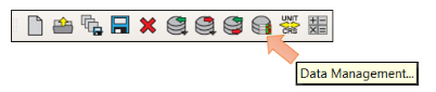
To reduce the size of a project, the user can use the Data management tool available from the general toolbar.
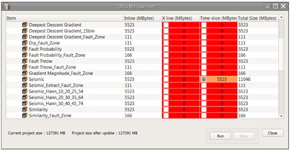
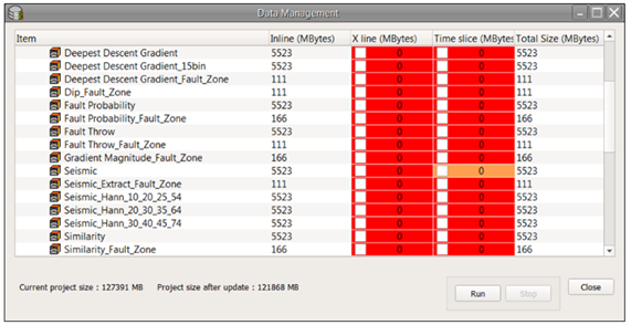
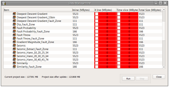
The Data Management tool is a table which quickly summarizes the X-line and Time Slice volumes and their sizes. The total size of the project is displayed at the bottom left corner of the window.
The volumes that have not been computed are in red. The already computed volumes are in green. The user has to check or uncheck the boxes to either compute or delete the associated volume. Finally, they can click on Run to launch the computations. Note that it is impossible to delete the Inline volume via this interface because all the other volumes (X-Line and Time Slice) are computed from the Inline one.
In the Project Data Exchange window, the current project is displayed on the left-hand side of the window, whereas the remote project is on the right-hand side. To display the remote project, the user has to select it from the pull-down menu. If the project is not listed, they can search for it using the Scan Projects button.Data can be transferred between the current project and a remote project. For the transfer of volumes, the user can check the Crossline and/or Time-Slice options to associate the X-line and Time-slide volumes in the copy. Items can be deleted from the project browser by using the Delete option (Red Cross).To transfer items, the user needs to select them and click on the arrows in the middle of the Project Data Exchange tool. When the process is over, a message is displayed at the bottom of the interface. Several items can be selected and sent to the other project simultaneously.


Data can be transferred between PaleoScan™ projects. This tool is useful to work on the local drive and then send results on a shared folder of the network. The Project Data Exchange tool is available from the general toolbar.

In the Project Data Exchange window, the current project is displayed on the left-hand side of the window, whereas the remote project is on the right-hand side. To display the remote project, the user has to select it from the pull-down menu. If the project is not listed, they can search for it using the Scan Projects button.Data can be transferred between the current project and a remote project. For the transfer of volumes, the user can check the Crossline and/or Time-Slice options to associate the X-line and Time-slide volumes in the copy. Items can be deleted from the project browser by using the Delete option (Red Cross).To transfer items, the user needs to select them and click on the arrows in the middle of the Project Data Exchange tool. When the process is over, a message is displayed at the bottom of the interface. Several items can be selected and sent to the other project simultaneously.

Remote Links:
A remote link corresponds to a symbolic link to objects (Volumes and Horizon Stacks) contained in another reference project. It is commonly referred to as “shortcuts” or “linked files”.
This kind of link is a faster way to exchange data between projects and can be used to launch local computations. Moreover, it allows reducing the size of the working project.
A remote link can be created from the data exchange tool. The option Volume Copy Mode has to be unchecked (default mode). Once the remote link is generated, the remote object is displayed in the project browser of the working project with a specific icon:

To physically copy a volume, the user has to check the option Volume Copy Mode in the bottom left corner of the Project Data Exchange tool.

To change the style of an object, the user has to be in selection mouse mode (F shortcut), then double click on the object to select it and then change the style of the object through the properties panel.
To display an object (faults, wells, markers, geobodies etc.…), this object has to be opened in the 3D viewer. Right click on the object in the Project Browser and choose “Open in 3D". The user can also drag and drop the object into the viewer or double click on it.
To do so, the user has to open a blending viewer and then drag and drop each volume. The transparency can be adjusted by moving the cursor up and down. This type of display is also available for arbitrary lines, horizons and horizon stacks.

The following shortcuts can be used:
Shift+C: close all the window
Shift+T: tile all the windows
Shift+H: horizontally tile all the windows
Shift+V: vertically tile all the windows
Shift+M: minimize a window
Shift+N: restore the window’s normal size.
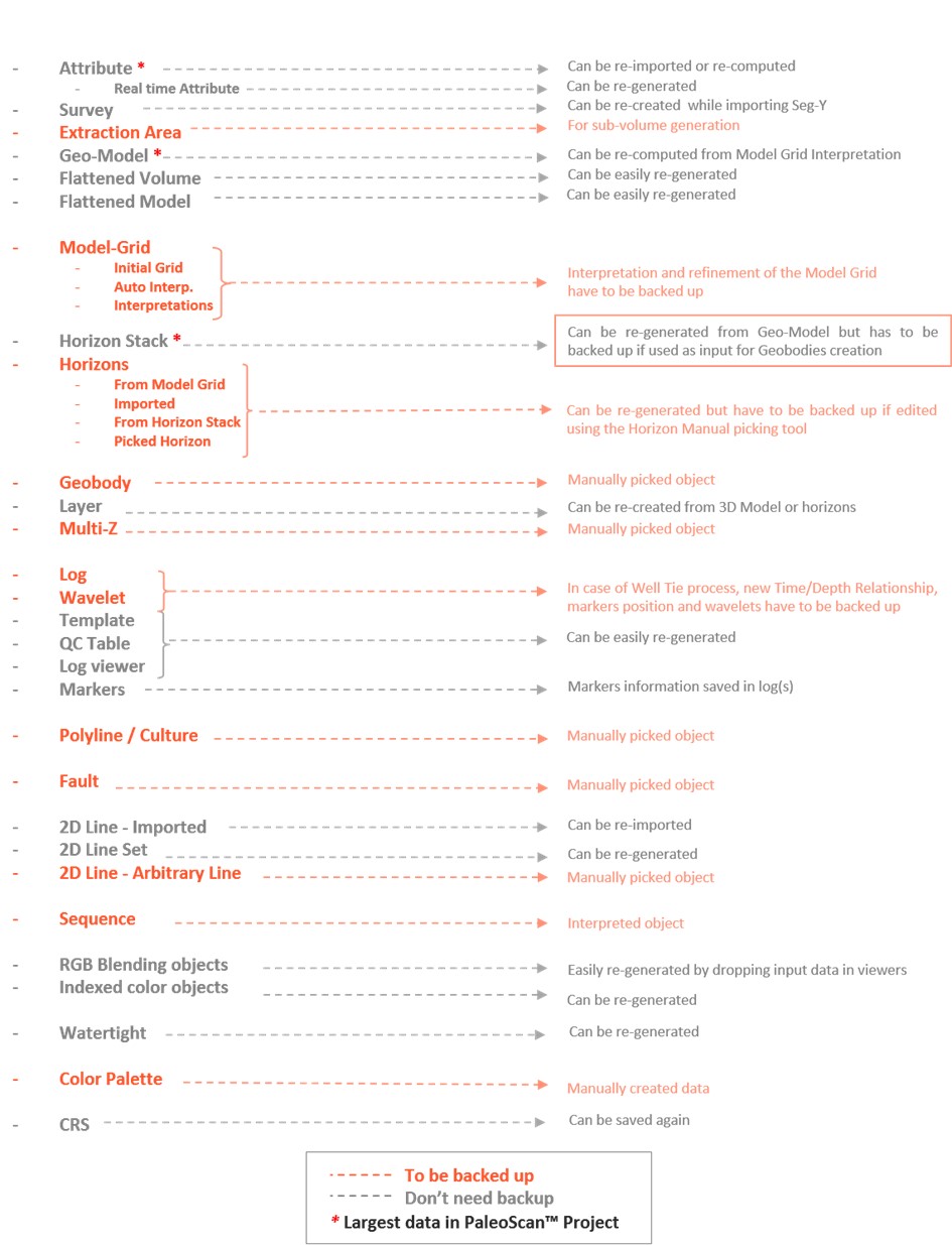
PaleoScan will automatically save all the imported data and all the calculated volumes.
All the objects created in PaleoScan need to be saved manually by the user.
The Model-Grids need to be saved using the Model-Grid toolbar save button. A back-up save is also automatically created every 100 propagations.

Faults need to be saved using the Fault tool bar save button. An emergency save is automatically created every 10 fault validations. The saving frequency can be modified from the settings.

Manually picked geobodies have to be saved individually. Multi-Z also need to be saved manually.
The user needs to drag and drop the seismic volume 3 times inside the 3D viewer, then select each section, using the selection mouse mode, (F shortcut) and change the Inline tab of the Volume Manager to Xline and Time Slice.
On a Time Slice, Horizon Stack or horizon viewer, the user can pick a polyline using one of the polyline mouse modes available from the main toolbar.

They can then select the polyline, using the selection mouse mode (F shortcut) and save it (CTRL+S) as a Polyline, 3D Polyline or Culture. It will be stored under the Polyline tab of the Project Browser.A Polyline is never displayed in the 3D viewer and is mapped on the selected Horizon Viewer or on the displayed horizon of a selected Horizon Stack viewer. This behaviour enables the geobody extraction.A 3D polyline is displayed in the 3D viewer but not on 2D viewers.A Culture is displayed at Z=0 in the 3D viewer and is snapped to every Time Slice and Horizon Slice in 2D view.
The user can use the buttons from the top toolbar to flip, rotate or stretch the displayed seismic section. The rotation and stretching can then be saved using the top toolbar or by right clicking on the top bar of the viewer.


From the 2D viewer, the user has to click on the Horizon Flattening option available at the bottom left corner of the window. To flatten along a horizon from the database, they need to drag and drop the horizon from the Project Browser into the Horizon drop zone and then click on OK. To flatten according to a horizon viewer, they have to click on Viewer as an input and then select the horizon viewer on which to flatten from the pull-down menu.
The flattening can be disabled or activated at any moment thanks to the OFF/ON buttons.

Model-Grid
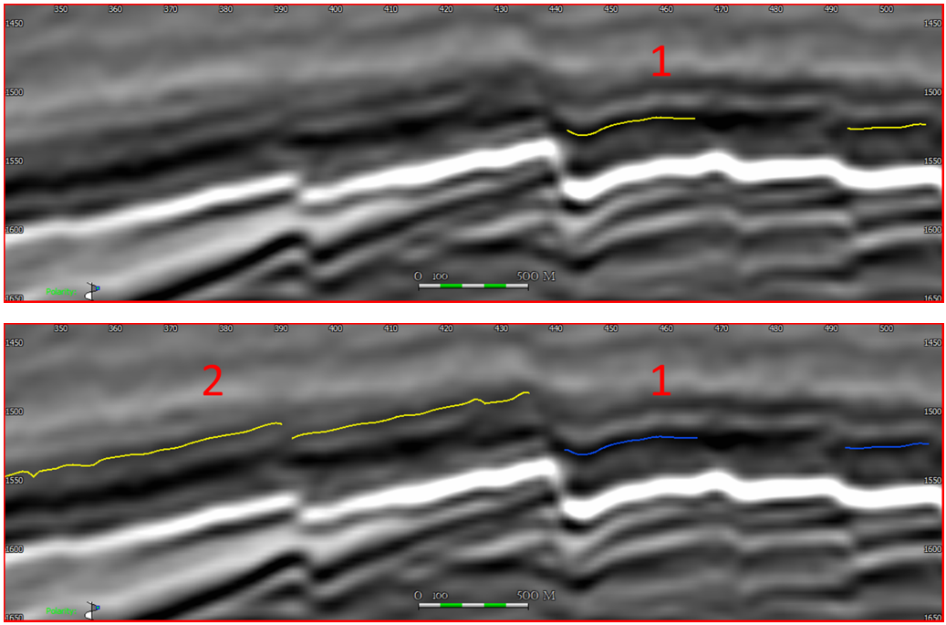
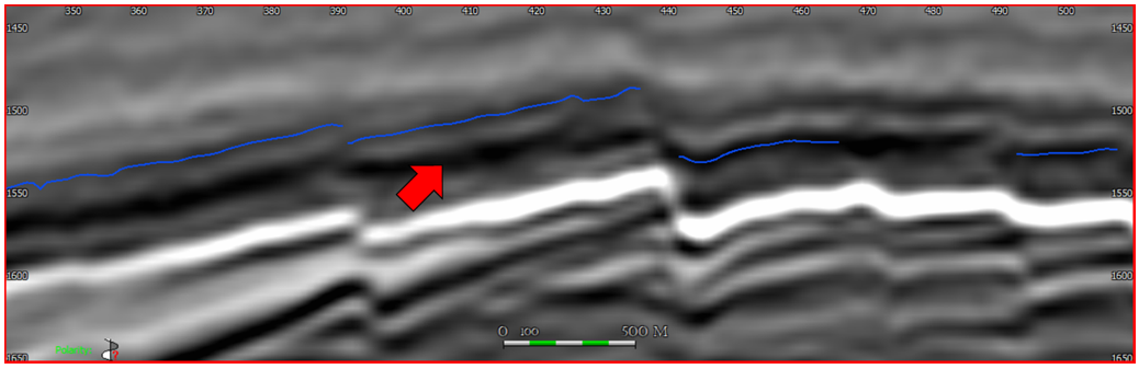
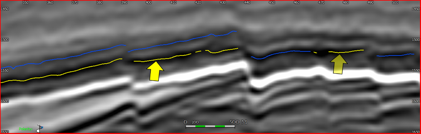
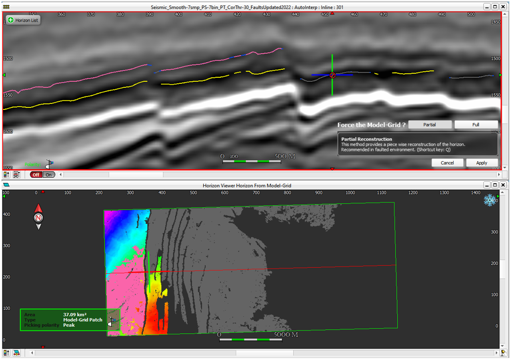
There are many ways to do that in PaleoScan. You could for example erase the wrong part with the eraser (by keeping pressing SHIFT and dragging your mouse on the seismic line or in the horizon viewer) and then connect normally to the right horizon patch. But it is not always needed to erase first. What we would recommend, is to activate the horizon you want to connect first, and then force the model grid to connect to the patch you're interested in following.
In this example, I've connected two patches (1 and 2) and created the "blue horizon" by marking it (by pressing "M" to validate and mark it with a color).
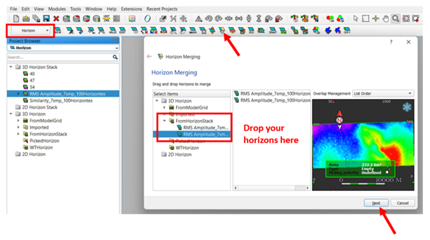
It is possible to update a model-grid with horizons coming from an old interpretation, Petrel or other applications.
Option 1: You could use the "model-grid constraint..." option. Use this option if the seismic is really similar (same resolution, etc), or else you may encounter problems. It is used, for example, on very wide seismic that has been split into several zones, in order to reuse the model-grid.
To use an existing interpretation as guide:
- First compute the New Model-Grid. It is better to use the same parameters than the one you will use as constraint (same patch size, polarity, etc)
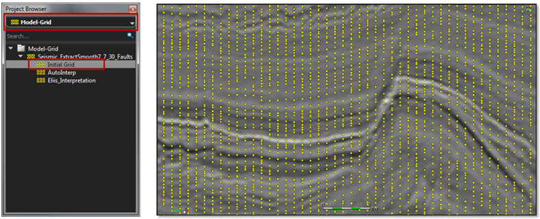
- Then Open the Initial Grid of this Model Grid
- Then insert the Model-Grid as constraint
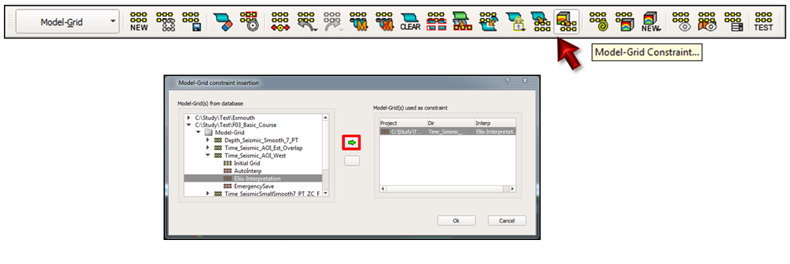
- Click on OK
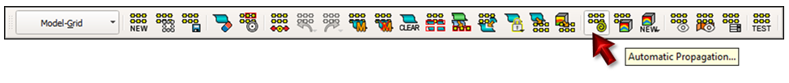
- When the Model Grid is inserted as constraint, don’t forget to re-compute an Automatic Propagation

- Finally Save your Model-Grid
Option 2: In this case, the workflow is almost the same, but you use the "Horizons as constraints" from your Initial Grid.
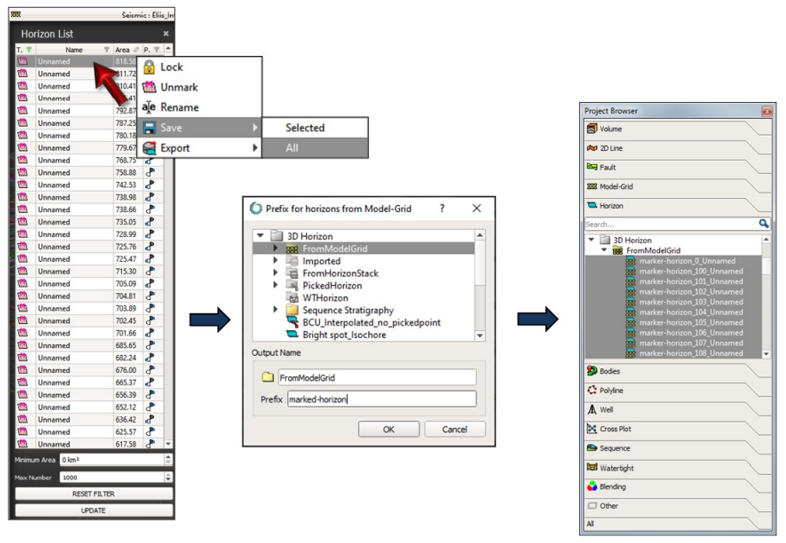
- First step would be to save the Marked Horizons from the Original Model-Grid as horizons and then use them to constraint the newer Model-Grid.
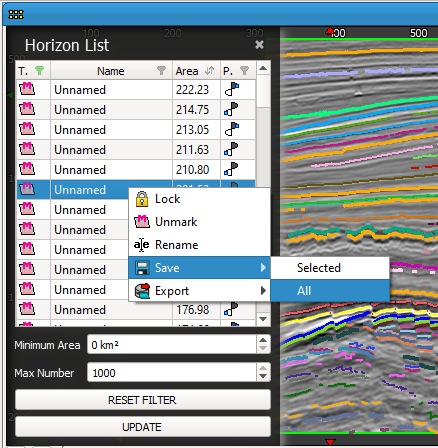
- Horizons can be saved using the Model-Grid Horizon list, right-click over any horizon and select Save/All.
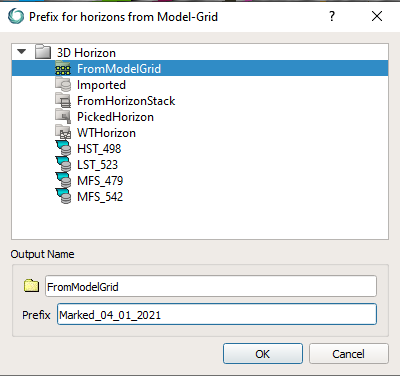
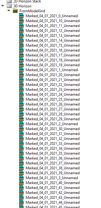
A prefix is asked to save several horizons at the same time. The Model-Grid horizons are stored and saved in the database under the Horizon tab.
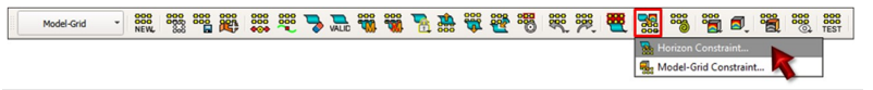
- Open the initial grid of your new Model-Grid. Use the option of Horizon Constraint. From the Model-Grid toolbar, select the Horizon Constraint option, or use the context menu of the Interp viewer and select the Horizon Constraint option:
- Select the horizons to use as constraints and drag and drop them into the specific area. The algorithm will link together patches that are in the vicinity of the horizon, respecting the selected parameters.
- When the horizons are inserted as constraint, don’t forget to re-compute an Automatic Propagation
I recommend checking the following Tips & Tricks video:
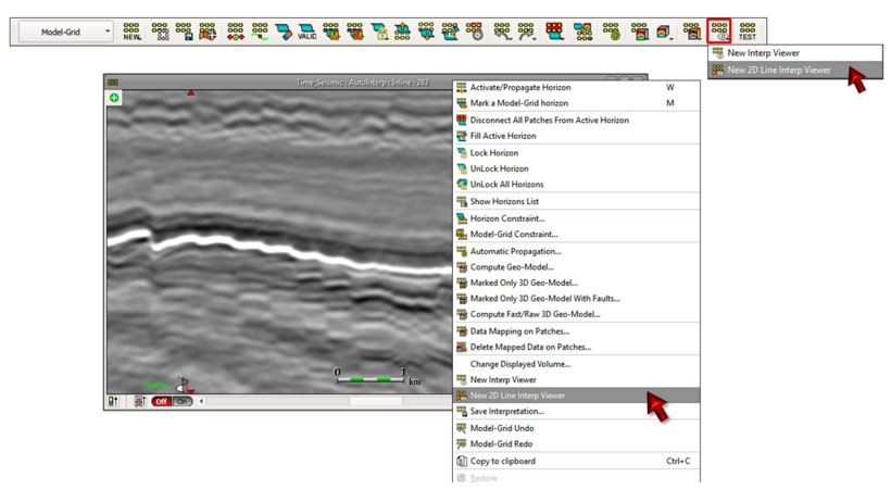
It is possible to visualize the model-grid on an arbitrary line. You will have to first create and save that arbitrary line. (Please, refer to the additional explanation at the end of this text, if needed). Then, once you have the Model-Grid open on an inline, you will be able to click on the “New 2D Line Interp Viewer” button in the Model-Grid toolbar or select the New 2D Line Interp Viewer option in the context menu of the Interpretation Viewer.
In the next interface, select the 2D line to use and click on “OK”.
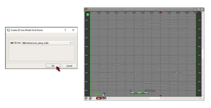
If the main interpretation viewer contains marked horizons, they will appear as well in the 2D line interpretation viewer. If a specifically marked horizon (or a patch) is activated through the 2D line viewer, this horizon will also be activated in the main interpretation viewer (and horizon viewer). You can go back and forth from one viewer to the other one and keep interpreting efficiently the data.
How to create an arbitrary line?
To create arbitrary line in PaleoScan, select the 2D Line module toolbar.
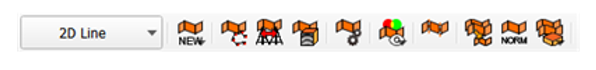
There are two options to create an arbitrary line:
Option 1: The first option aims at creating an arbitrary line based on the positions of wells.
- Click on the third button starting from the left
 New Arbitrary Line Along Wells. In this application, you will first need to drag and drop the wells you wish to use to define the path of the arbitrary line.
 - Drag and drop the volume to extract along this line.
- Once done, click on the following button Search Optimum Trajectory located in the middle of the application. PaleoScan will this way find the best trajectory along the selected wells.
- Finally, if you wish to save the arbitrary line, define an output name and click on OK.
Option 2: The second option aims at creating an arbitrary line based on a random polyline.
- Open a horizon viewer, or seismic line and display it as a time slice using the Volume Manager.
- Click on the first button of the 2D Line toolbar New > Arbitrary Line Creation.
- Now you will have a specific mouse mode that allows you to pick the trajectory of the arbitrary line in the horizon viewer/ time slice viewer. Double click for ending the picking of the trajectory.
- An application should pop up.
- Select the volume to extract along the line and click on next. If you wish to save the line you will need to define an output name and click on OK. If you already have an arbitrary line in your project, you can display it in a map, select it and click on the second button of the 2D Line toolbar New Arbitrary Line from Polyline. You will skip the 3 first points of this workflow. The following steps are the same.
For both options, the arbitrary line saved will be stored under the 2D Line tab of the Project Browser.
In PaleoScan, you can also generate a 3D iso-proportional Geo-Model using only few horizons.
It interpolates between horizons coming from external interpretation.
To do it, you should go to Horizon module and select the "Geo-Model from Horizons" option, then "3D Geo-Model from Horizons".
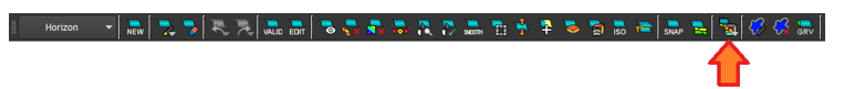
1- Drop a volume as input.
2- Drop all the horizons or a horizon stack to be used for the iso-proportional 3D Geo-Model computation.
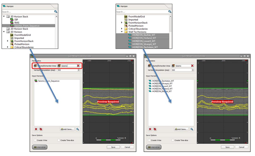
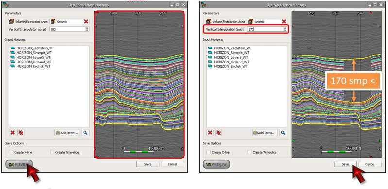
3- Launch the preview by click on the Preview button and adjust the vertical interpolation size (expressed in smp) if needed. Then, click on Save to generate the iso-proportional 3D Geo-Model which will be saved and stored under the Model folder of the Volume tab.
In this example, if we use a "Vertical interpolation (smp)" of 170 smp, then we will see gaps where the vertical distance between two horizons is greater than 170 smp.
This is an issue that deals with the maximum number of patches that the software is going to make when building your model-grid.
Here is what you can do to remedy this.
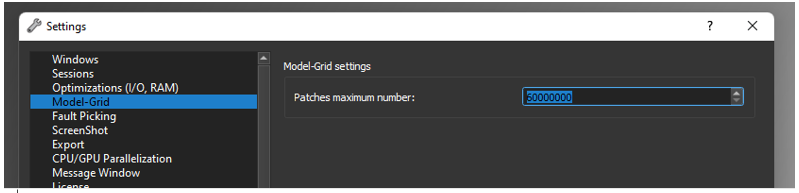
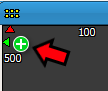
Depending on the version of the software you are running you can increase the maximum number of patches the software will make up to 1 billion. By default, it is set to 60 million in the settings menu but you can increase this number by following these steps:
a. Open the settings menu
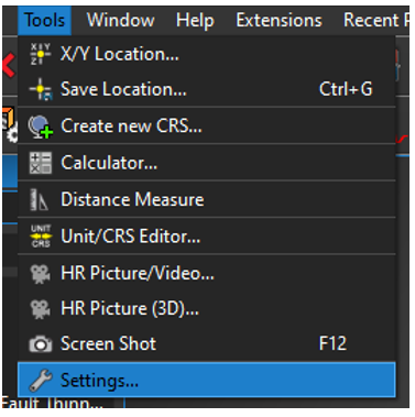
b. Click on "Model-Grid" and increase the number of patches to 100 million or 500 million, etc...
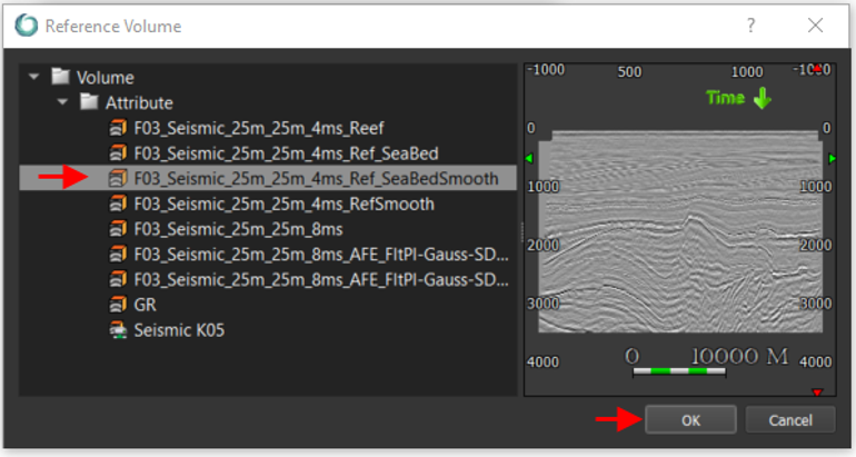
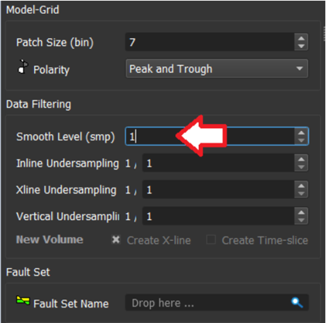
The reference volume associated to your Model-Grid can be replaced/reassigned. Hence, even though you have deleted this volume, you can recreate it from the initial seismic volume applying the smoothing you want and eventually reassign this volume as the Model-Grid reference volume. To do so, please follow these steps:
1. From the initial seismic volume, reapply the smoothing you want: 'Volume' toolbar > 'Volume Attributes' button> '3D Smooth Gaussian' then enter as Input your initial seismic, and as parameters thrice the same value for the In-Line, X-Line and Vertical Smooth (the default value of this smoothing when you create a Model-Grid is 7); click "Run" to compute the smoothed volume
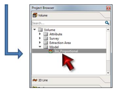
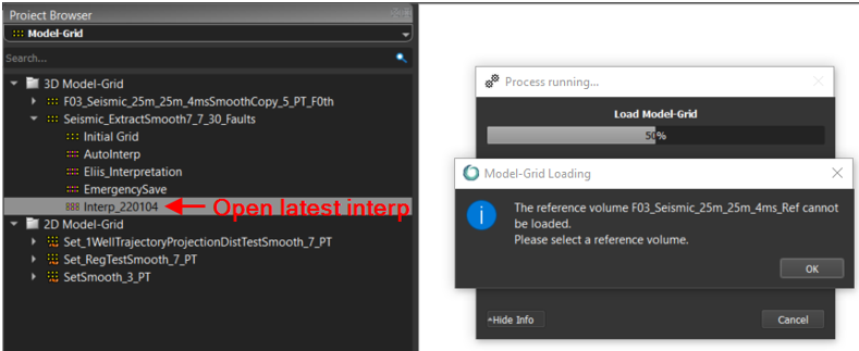
2. Reopen your Model-Grid interpretation and reassign the newly recreated smoothed volume as the Model-Grid reference volume: Project Browser > 'Model-Grid', then select the Model-Grid whose you deleted the reference volume and double-click to open your latest interpretation. At this point, PaleoScan will start loading the grid, recognize that the reference volume is missing and propose to select a new one. Click "OK" then, in the displayed list, select the newly recreated smoothed volume. Click "OK" and the Model-Grid with the preserved interpretation will be displayed again.
The interpretation in the Model Grid is polarity consistent, by default, the interpreted horizons cannot have polarity changes.
Nevertheless, the user can manage unconformities with polarity changes by disabling the "polarity consistency" option in the Properties of the model grid.

The preview is done using a couple of constraints around the yellow seed while the real geomodel uses all the constraints present in the entire grid.
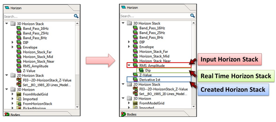
The horizons coming from the Model-Grid are seismically consistent and present where there are data. In the case of erosion or non-deposition, the horizon will not be mapped. It is geologically consistent.
The horizons coming from the Horizon Stack are modelled through the Geo-Model, meaning they are smoother, covering the entire survey, even in the case of erosion or non-deposition, and following the trend of the seismic. They are no longer seismically consistent.
Not necessarily, even if there is a gap in the marked horizons. By increasing the interpolation parameter for the Geo-Model creation, PaleoScan will fill the gaps and the Horizon Stack will be complete (if the Interpolation Size is high enough).
To rename a horizon from the Model-Grid, the user has to open the Horizon List, right click on the name and select the option Rename.

The horizon can also be selected (F keyboard shortcut) by double clicking on the horizon in the Model-Grid (the horizon turns red), it can then be named from the Properties window.

Having gaps in the preview does not mean having a lack of nodes, it just means that the nodes inside the gaps are not linked to the rest of the Model-Grid. To address this issue, the user needs to connect nodes inside the gaps to nodes outside the gaps (i.e. where there is a preview).
If there is a gap in the preview that the user cannot fill, increasing the interpolation parameter in the Geo-Model Creation window will help fill the gaps in order to have a complete Geo-Model.
To refine the grid, the user needs to be in cross navigation mouse mode (G shortcut). They then need to place the seed on a specific event and press W to activate the chosen event. Next, they have to place the yellow seed on the belonging event and press W again, PaleoScan will connect both horizon patches. This action can be repeated as many times as needed to extend the current horizon as desired.
Once the user is done with the horizon refinement, they can click on the space bar to validate or on M to mark the event.
It is possible. To do this, the user needs to open the Model-Grid and click on the Grid Constraints and then Model-Grid Constraint icon and follow the workflow.

The user needs to make sure to start from the initial Grid (and not the AutoInterp). This ensures that the constraint from the horizons will be applied to a "blank canvas", and that there will not be any conflict.

They need to add the horizons to be used as constraints for the Initial Grid using the Horizon Constraint button.

Finally, they have to re-run an auto-interpretation using the Automatic Propagation button in order to take into account the horizon inserted as constraints.

The user has to keep in mind that if the horizons used as constraints are not single-polarity, PaleoScan may give results that are not consistent with the first interpretation.
To save or extract a specific horizon the user needs to mark the horizon, then select it using the Selection Mode (F shortcut) and click on the blue floppy disk in the top toolbar or use the keyboard shortcut CTRL+S.

The grid can be generated between two horizons, or from the top/bottom of the seismic to the key horizon. The option is available in the Advanced Options of the Model-Grid Creation tool.

The input horizons need to be continuous where the Model-Grid is to be generated: no node will be computed between a hole (=void) and a surface, or a hole (=void) and another hole (=void). The Propagate/Interpolate tool available from the Horizon toolbar can be used to fill existing gaps or to generate full surfaces from a picked horizon.
In order to properly interpret and model the stratigraphic level of interest, it is strongly advised to shift both the upper and lower boundaries of +/- 100 to 300ms. This preliminary data conditioning can be done using the Vertical Shift tool available from the Horizon toolbar.
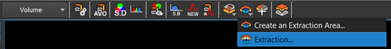
A cropped seismic volume can also be created. Using the Extraction tools available from the Volume toolbar, the user can create an extraction area and then extract this sub volume from the original one. The Model-Grid can then be created on this cropped volume.
Yes, to re-edit a marked horizon, the user needs to activate the cross-navigation mouse mode (G shortcut), put the seed on the marked horizon and press W. The horizon can then be edited as desired.
In the Advanced Options of the Model-Grid creation tool, an Exclusion Zone(s) parameter allows the user to drop objects (layers, geobodies and Multi-Z) so that PaleoScan will not create nodes inside those objects.

The nodes display is a projection when the seismic section is not located exactly at the centre of the patch. Therefore, the nodes might be slightly shifted compared to the seismic events. The patches, which define the horizons, will follow the seismic events anyway.
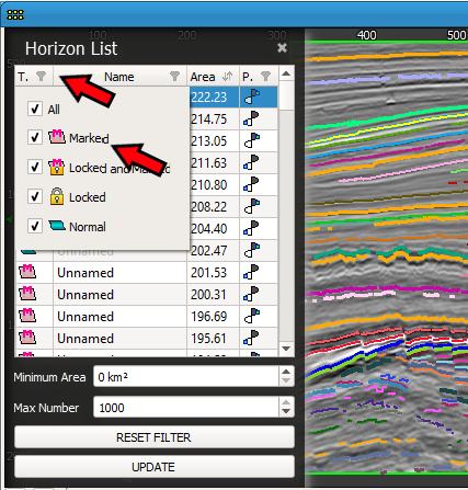
The user needs to click on the Update button at the bottom of the horizon list to refresh it. The marked horizons will appear with a M


If faults and/or exclusion zones were used for the Model-Grid generation, there will be voids at the location of the faults/exclusion zones. This is quite useful if the user does not want to generate the grid around salt domes for instance. If the user wants to have nodes at these locations, they must not use the faults/exclusion zones option.
A marked horizon is a horizon that the user decides to highlight using the M keyboard shortcut. It is displayed in colour. However, it is not a saved horizon. Horizons that are not marked are also taken into account and validated by pressing the Space bar. All horizons, marked and not marked, will be used to calculate the Geo-Model.
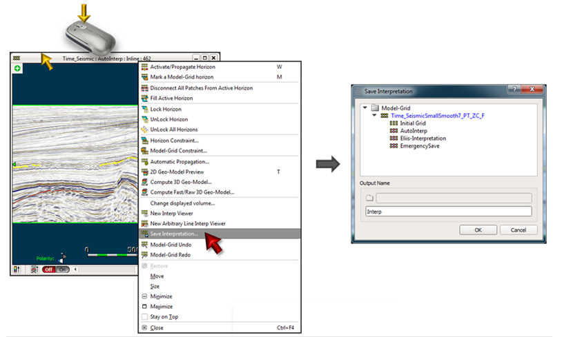
The global interpretation needs to be saved using the top bar of the Model-Grid window or the Save Interpretation button of the Model-Grid toolbar.
Horizon stacks
To display two horizon stacks from different blocks in the same window, you have two options:
• First Option: Open both horizon stack in a 3D viewer. Select each of them (by double clicking on it with the white arrow) and scroll to reach the horizon of interest. To have a better view, use the Top view tool:
You can do the RMS on a dynamic window (between horizons) in PaleoScan.
It is not possible to compute the RMS between horizons in the Horizon Stack but it is possible to do it between Horizons.
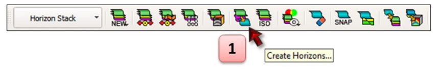
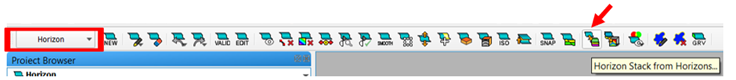
• Firstly, you must extract the horizons you are interested in from your horizon stack. To do that you can use the tool ‘’Create Horizons…’’  in the module Horizon Stack.
• Then, you can open the horizon on which you want to map the RMS. And, in the module Horizon you can use the tool ‘"Attribute Mapping on Horizon’" , choose the RMS, check the option "Dynamic window size" and finally chose the dynamic window you want for the RMS.
and double click in the Horizon Viewer. Once the horizon is selected a red square will appear around the viewer. in the main toolbar and chose the name of the horizon. Attributes can be mapped on an existing 3D Horizon Stack. It allows generating the same Horizon Stack as the input one but with another attribute.
The Duplicate Horizon Stack with new Attribute tool is available from:
a/ Project Browser context menu, as Duplicate option
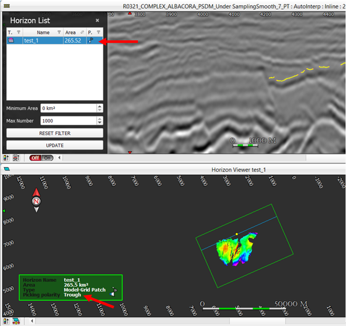
To save the marked horizons out from the Model-Grid, you can use the Horizon List to filter by "Marked Horizons" type and save them all at the same time.
1- You can open the Horizon List by clicking the green + sign in the upper left corner of the Model-Grid window:
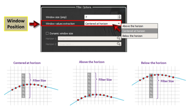
The "Window Size" parameter of the Horizon Stack, and any other horizon extraction, will depend on the input seismic volume (and not on the GeoModel vertical resolution). Moreover, the "sample" will depend on what domain your seismic volume is from. For example: if you are working with a seismic volume in time with a sampling rate of 2ms, then, a "Window Size (smp) = 7" will correspond to a 14ms window. Likewise, if you are working with seismic data in depth with a sampling rate of 10ft, then the same Window size of 7 will correspond to a 70ft window.
You also have the option of selecting the "Window values extraction" to be Above, Centered, or Below each horizon (In the following cartoon, each Xn represents a sample)
When you are working in the Model-Grid, it is possible to work with single polarity horizons and multi polarity horizons.
When the horizon has multi-polarity, the “Undefined" polarity is given.
Unfortunately, there is no way to know which part of the horizon is a peak or a trough, in order to erase it.
The workaround would be:
1- Save the undefined polarity horizon (F + double on it then CTRL+S). It will be saved in the 3D HORIZON folder, under the "from model grid" sub-folder.
2- Use this horizon as a constrain selecting the single polarity option:

3- PaleoScan will use the polarity that is the most present on the horizon. Click on OK.
Once the horizon is inserted in the model-grid, it will appear in the horizon list. You will be able to see the polarity there or in the green square in the horizon viewer.
It is fixed!
Even though the "Truncation" mode is applied in the Strati Viewer and the "Edit/Create a GeoModel from Sequence" tool is used, the model produced shows condensed time intervals. Unfortunately, there is no way to create strictly truncated models.
Because of the above technical limitation, you cannot rely on a model to output Horizon Stack/Horizons where the horizons would be truncated according to geological truncations.
That being said, here is the way to extract truncated horizons (in a Horizon Stack) out of the Strati Viewer:
1. When in the Strati Viewer, use the "Strati Sequence Picking" tool [J] to
a. Create layer boundaries corresponding to the unconformities in the seismic interval of interest,
b. Then create between the unconformity boundaries as many boundaries as desired horizons in the Horizon Stack you envision to create (do not use the Properties > Sub-layering option relative to the created layers). Color code does not reflect different types of boundaries but just for step understanding purpose.
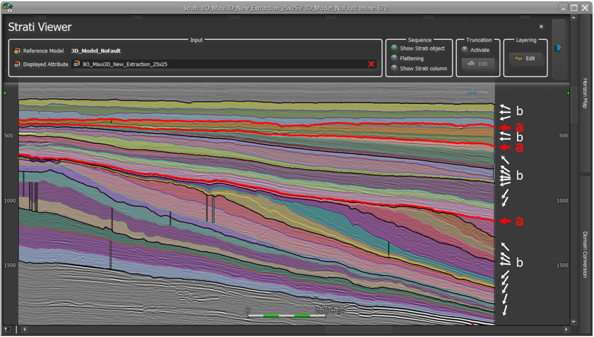
2. After having checked the "Activate" Truncation mode
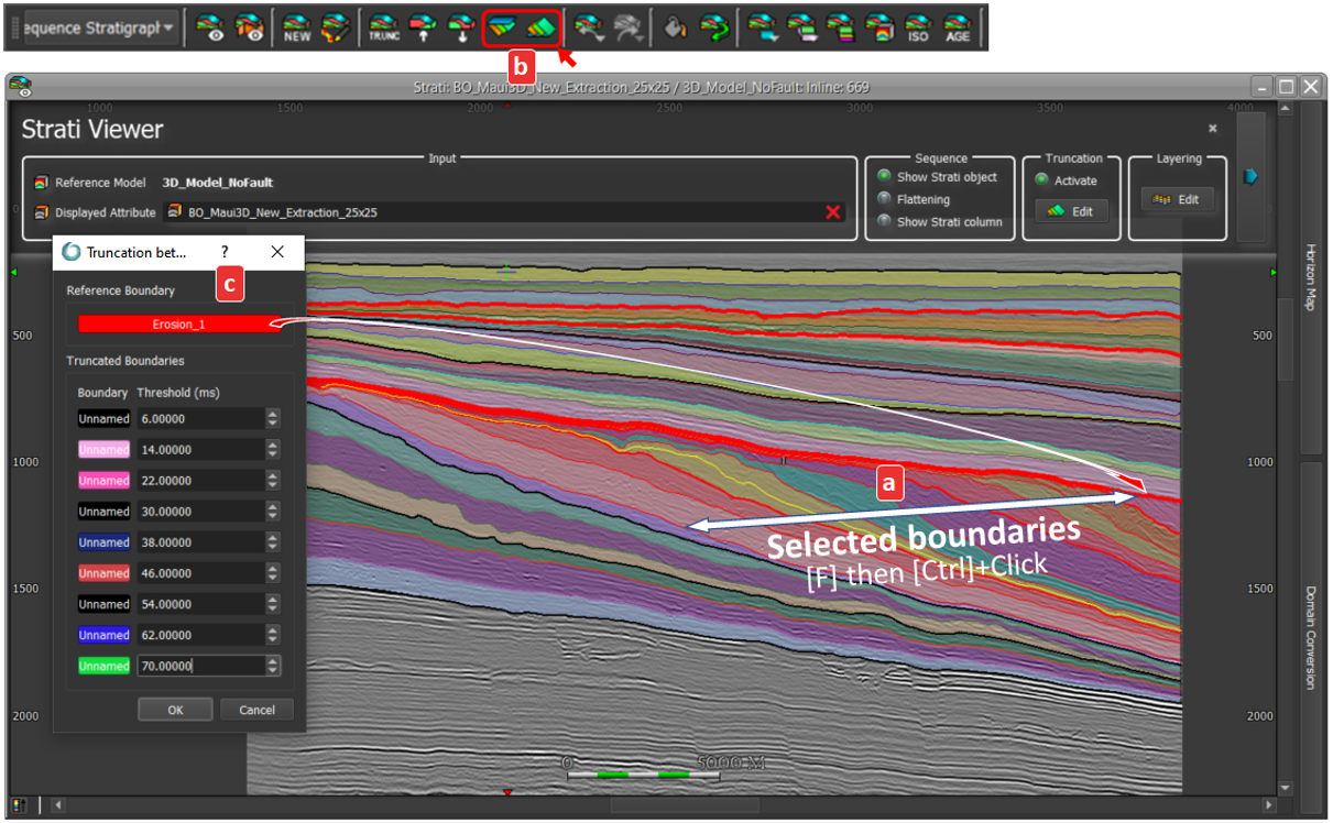
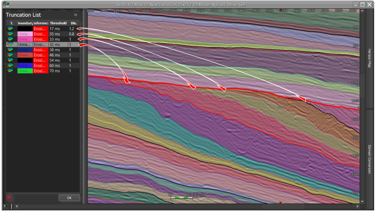
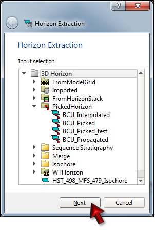
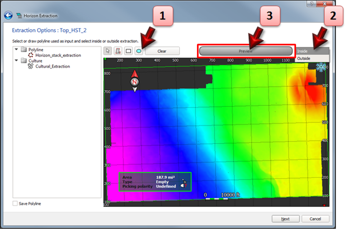
You need to use the Horizon Extraction tool:
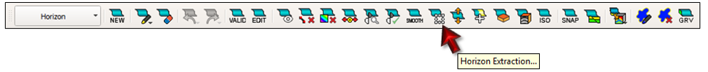
- The horizon to extract must be chosen within the data base.
2- Then the extraction options must be checked.
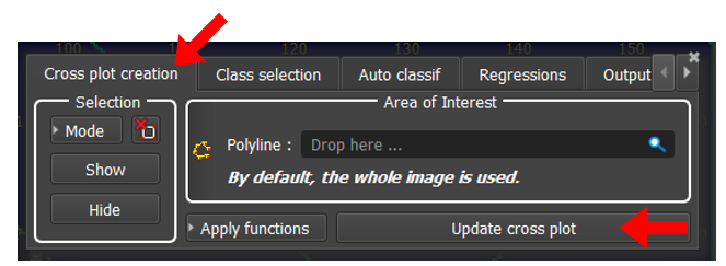
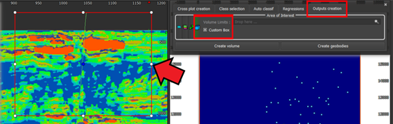
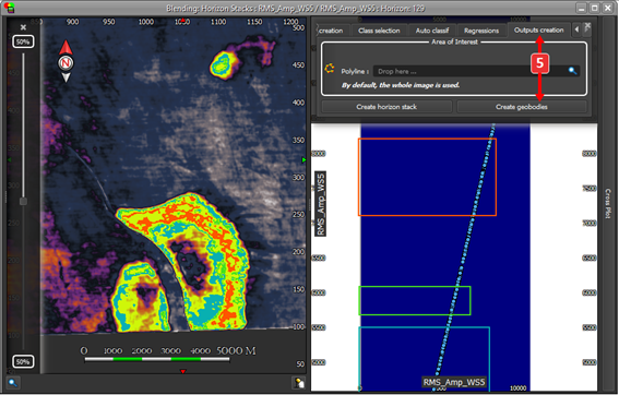
The area of extraction must be defined. A pre-existing polyline intersecting the horizon, or a culture data can be selected. A new polyline can also be created. Any area of extraction can be cleared from the viewer. The inner or the outer part of the area can be extracted. By toggling on the “Save Polyline” option, the current picked polyline can be saved in the database. It will be saved under the “Polyline” tab of the Project Browser.
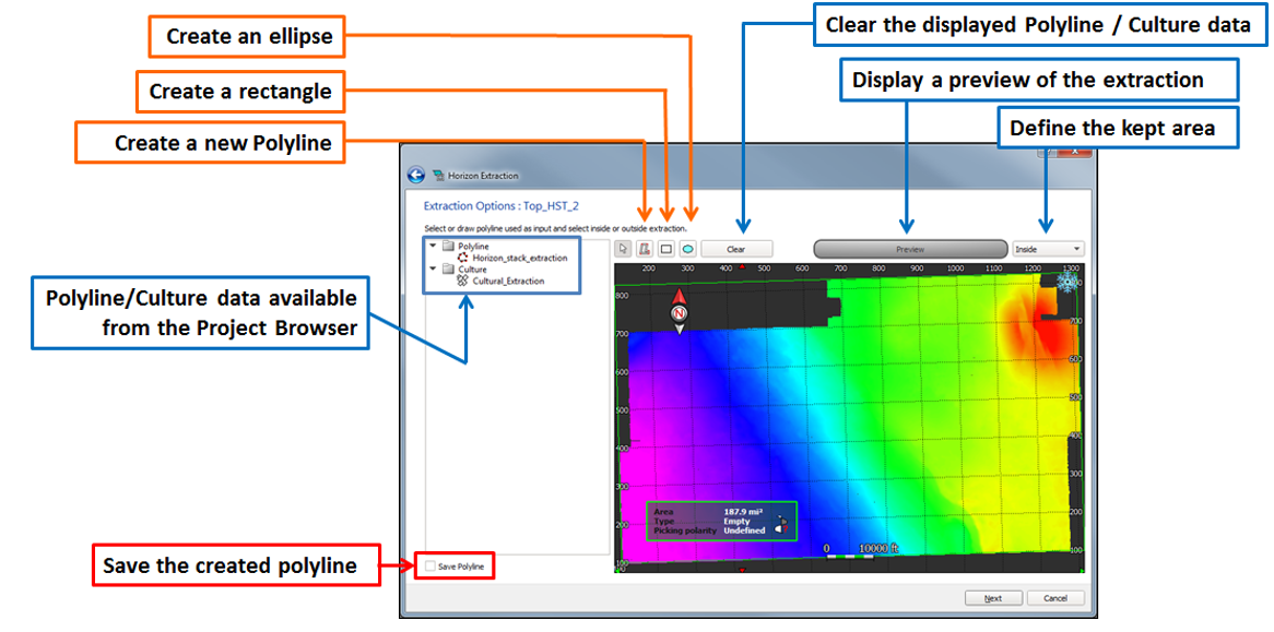
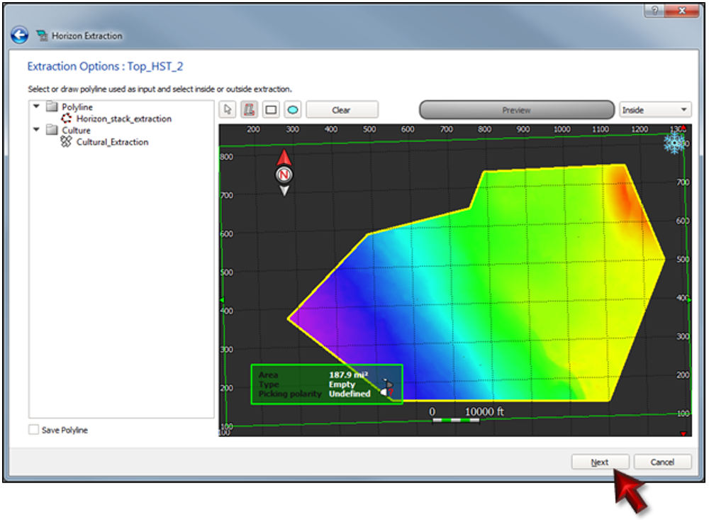
3- Once the area of extraction is defined, click on “Preview”.
4- The preview of the extraction is displayed. Then click on “Next”.
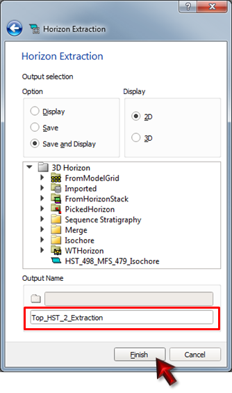
5- Select the output options. Enter a name for the extracted horizon in case of saving. Then click on “Finish”. In case of 2D display, a Horizon Viewer is automatically opened with a survey (green frame) related to the original horizon.
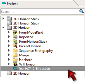
6- Once saved, an extracted horizon is stored within the Horizon tab of the Project Browser. This new horizon can be opened in a 2D or 3D viewer. If it is opened in a 2D viewer, the survey (green frame) displayed within the map view is automatically adjusted to the edges of this horizon.
When the Horizon Stack is computed directly from the Geo-Model, it is not possible to choose the horizons that will make up the Horizon Stack. The user can only choose an interval, the number of horizons and the attribute(s) to map.
Nevertheless, the user can choose all the horizons of the Horizon Stack if it is computed from the Sequence Stratigraphy toolbar (available in the Advanced Interpretation add-on module), using the New Horizon Stack from Sequence tool. In that case, the user can define the limits of the sequences within which the Horizon Stack will be created.

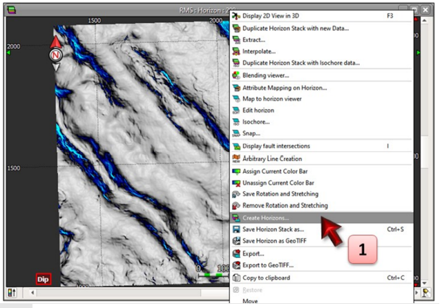
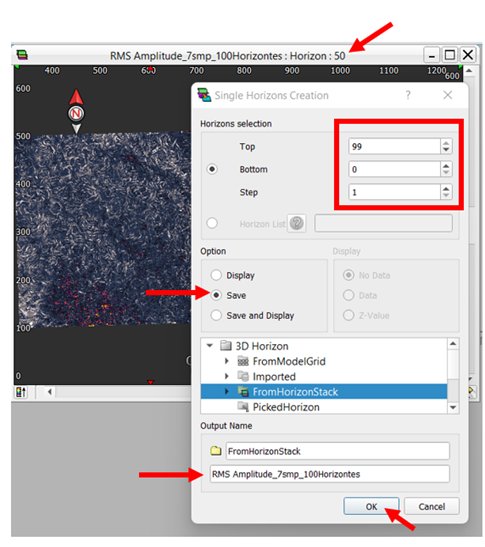
To save or extract a specific horizon from a Horizon Stack, the user has to right click on the top bar of the Horizon Stack viewer and select the option called Create Horizon(s). By default, PaleoScan will save and extract the currently displayed horizon, but a top, a bottom and a step can also be defined to save and extract a set of single horizons.

Faults
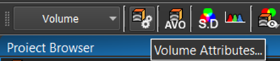
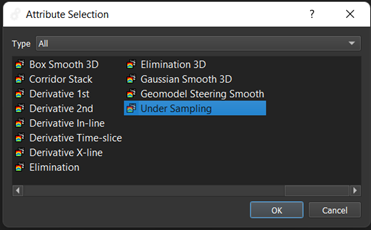
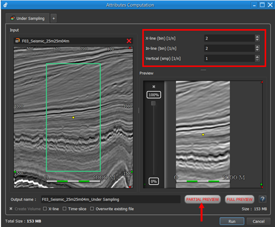
1. You could under sample your data vertically. It will reduce the size and hence reduce the computation time. You can either apply this during the initial import or after from the volume attribute icon.
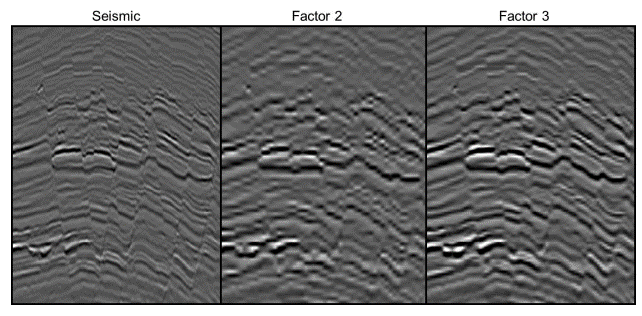
We strongly recommend properly conditioning the data by clipping, under sampling/decimating it according to the dimension of signal discontinuities to emphasize (towards fault extraction).
The following picture shows the results of the under sampling applied on a volume with two different under sampling factors.
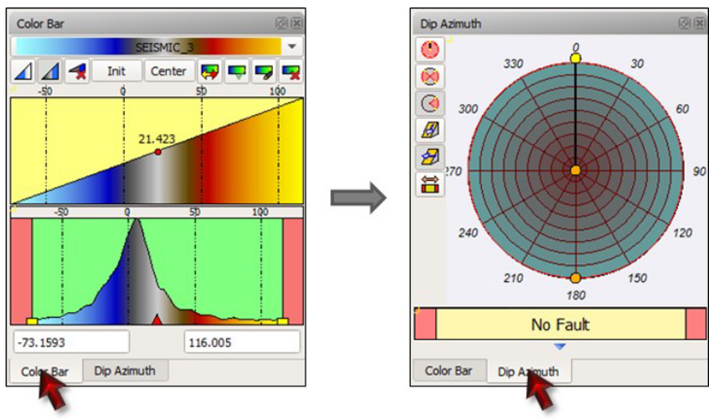
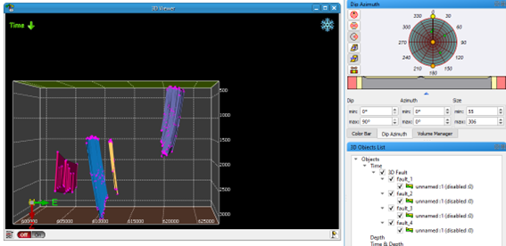
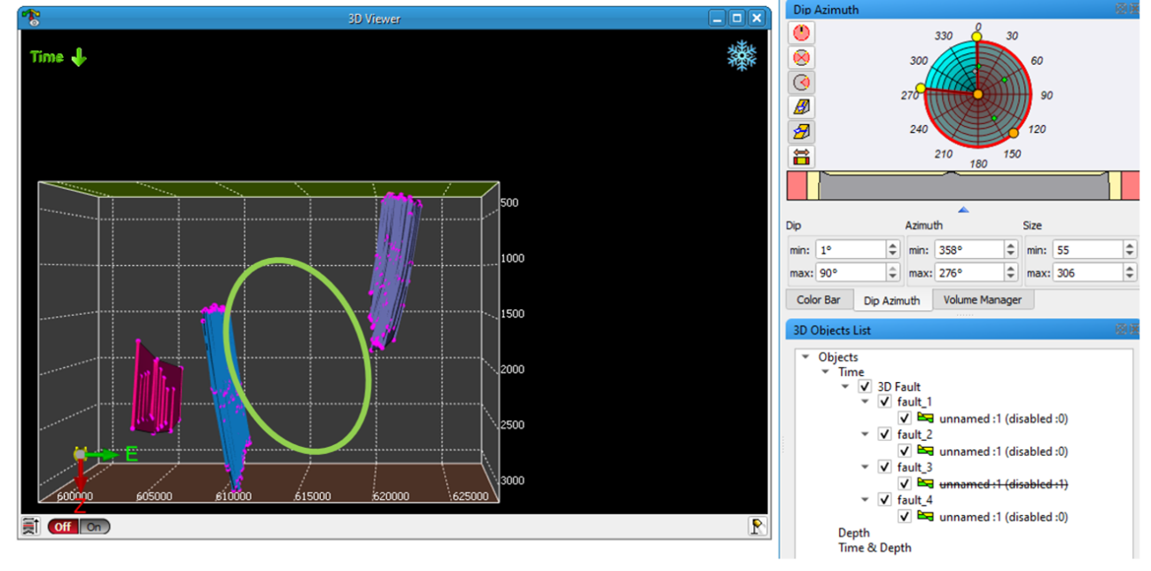
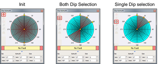
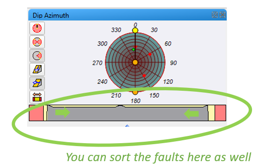
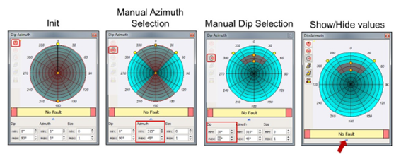
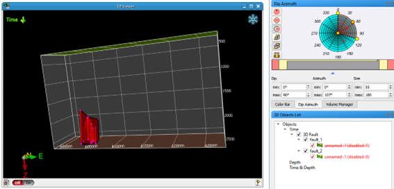
The Dip Azimuth Filter allows you to get rid of some faults (or segments) based on the Dip/Azimuth and size.
It is located behind the color bar dock widget:
Once created, it is possible to modify your newly created fault set, even if you have already validated the faults.
Once picked, you may add some, delete them, move anchor points, merge or split them.
There are several options in the "Fault" toolbar that you can use.
• The 15th and 16th buttons: Faults Merging (Shift + Q) & Fault Splitting (Shift + W)

If two or several fault patches belong to the same geological fault, they can be merged.
The merging tool will create a single fault based on several patches.
To do so:
1/ Select the 1st fault (by double-clicking on it)
2/ Keep holding down the CTRL key and select all the other faults to merge
3/ Selected faults should appear in red
4/ Click on the "Fault Merging" button
The splitting tool will un-merge faults that have been previously merged.
1/ Select the fault
2/ Click on the "Fault Splitting" button. All the original patches will be restored.
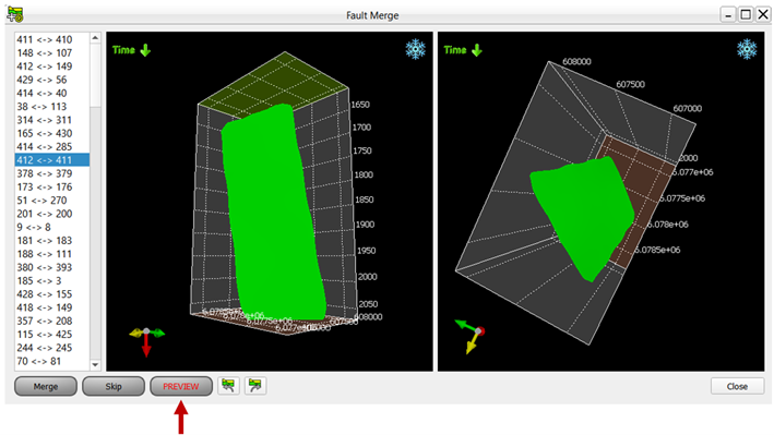
The "Fault Merge Assistant" is useful to find and merge faults across the entire survey area.
Click on the 17th icon button in the Fault toolbar (which works only from the faults visible on the 3D viewer).

The Fault Merge Assistant sorts the merges from the most probable merge to the less probable merge (as a function of: the distance between faults, dip/azimuth compatibility of the fault planes and the connection quality between fault borders).
If you want to merge faults:
- Open the assistant
- Click on the faults to merge
- Preview the merge
Once created, it is possible to modify your newly created fault set, even if you already have validated the faults.
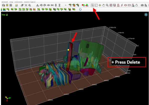
1/ To delete a fault from a fault set:
- Open the fault set from your project browser.
- Select the Selection mouse mode (shortcut F)
- Select the fault you want to delete by double-clicking on it.
- Press Delete from your keyboard
- Not mandatory: Open the fault set from your project browser
- Open a seismic section. (You should see the intersection of the faults with the seismic if you opened the fault set)
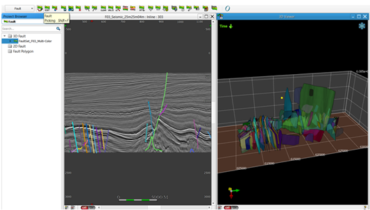
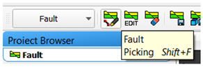
- Click on Fault picking
- Pick your fault, validate it.
- Now your new fault has been created in a new fault set. To add this new fault to the other one, follow the following step:
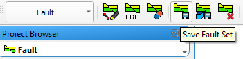
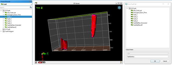
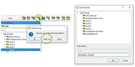
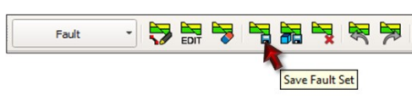
Here are some recommended steps to create a new and single Fault Set in PaleoScan to be used as a constraint in the Model-Grid computation:
1- Make sure to remove all faults from the 3D object list (right-click on them and click on Remove): This is to avoid any confusion with previous faults in the 3D object list.
2- Select all the faults from your project browser and open them in the 3D viewer.
3- Then, click “Save Fault Set” icon in the Fault module. This will select all faults in the viewer (turning them red) and will ask if you would like to save them all in a new fault set.
Yes, when the user starts picking a fault in the Inline direction, they can keep picking the fault in other directions such as Xline, Time Slice and even on Horizon Stacks.
Yes, it is possible to merge two or more faults using the Faults Merging/Splitting tools available from the Fault toolbar. It is also possible to split a fault which has been previously merged.

Yes, the user needs to click on the EDIT icon of the Fault picking toolbar and then double click on the fault you wish to edit. You can add, move or remove fault sticks.

PaleoScan can deal with reverse fault by generating two horizons for the same event. In case of a steep dip, everything works fine. In the case of a low angle fault, PaleoScan can handle the reverse fault if there is a low throw.
Volumes & Attributes
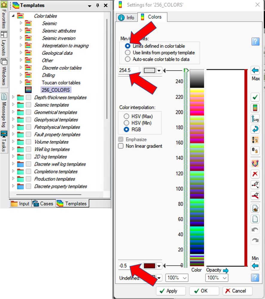
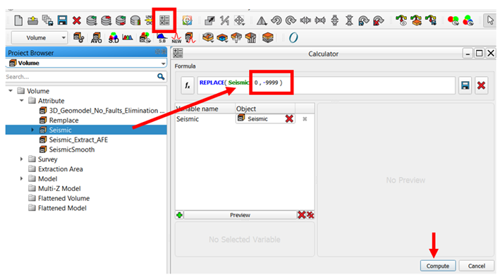
The "squeeze" of the color bar comes from the many dead traces in your seismic: where there is no acquisition, a 0 value is allocated.
You have two options to deal with this issue and restore your color bar.
If your segy is encoded in 32bit, feel free to use the following workaround :
- Open the calculator.
- Use the “REPLACE” function: Write “REPLACE”, drag and drop your seismic for the first variable, write 0 for the second one, and -9999 for the third one.
- Hit Compute.
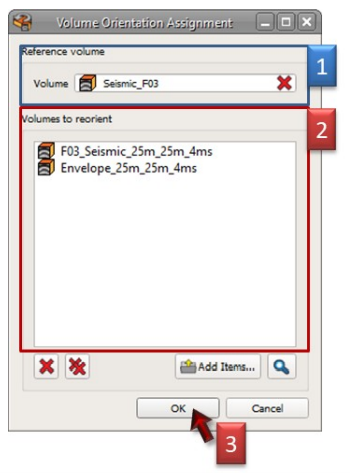
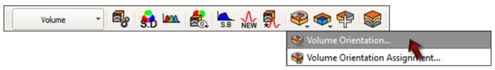
Several volumes can be oriented using a reference volume. All the input volumes will have the same orientation as the reference volume. Click on Volume Orientation Assignment in the Volume module to open the interface.
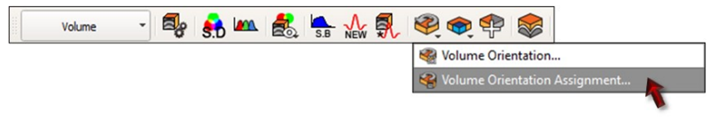
1. Drag and drop the reference volume,
2. Drag and drop the Volume(s) to reorient,
3. Click on “OK”.
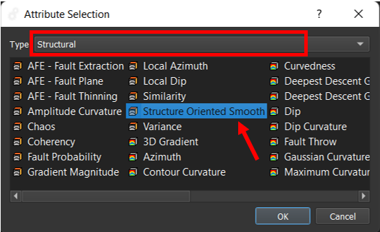
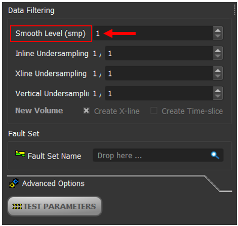
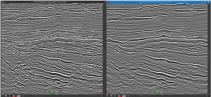
The Structure oriented smooth attribute offers a smoothing steered by the dip of the seismic event. In practice, a 3D vector field is computed with the defined parameters in the whole seismic cube and the smoothing is then applied following the directions of this vector field.
The parametrization highly depends on the data itself and unfortunately there is no rule of thumb.
1- Open the 3D attribute list from the volume module
2- Select the structured oriented smooth attribute
3- Adapt the parameters and test them using the preview. PX means pixels and it spatially represents the traces and vertically the samples. Then hit the Partial Preview icon. PaleoScan will run a quick SOS around the location of the yellow seed and display it. To enlarge this preview window, you can activate it by clicking in it, and from the properties panes you can modify the Width and Height values.
The issue happens when the remote link is broken (deleted object from the master project for example). It will not be possible to delete directly the linked object.
However, you could easily delete it by doing this:
1- Double click on the linked volume
2- Select a volume inside a project (PaleoScanProject/Volume/Attribute)
3- Close the volume window
4- Right click on the linked volume
5- Delete it
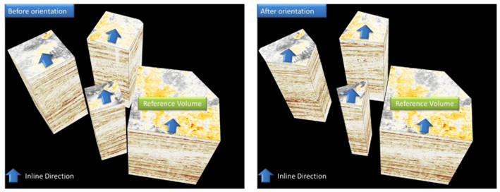
You can rotate your seismic volume in your preferred direction. Volume Orientation tool is in the Volume Module:
Then you can select the volume to orient and define the new direction for it using the Orientation Preview:
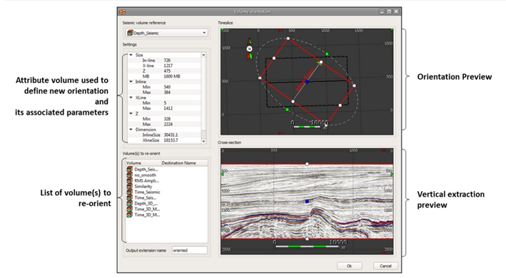
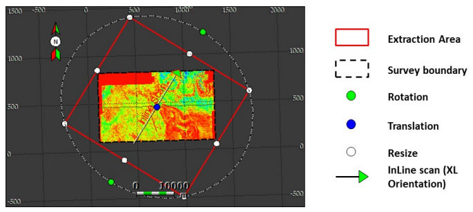
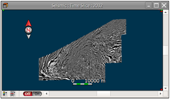
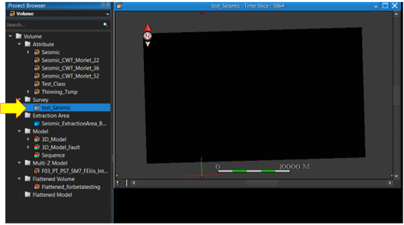
If you don't have the Time Slice, the seismic survey is the black dash line in the Orientation Preview. You should make sure that the rotated extraction area (the red outline in the preview) should cover the whole seismic survey or the time slice to avoid any data cropping. Then you click on 'Ok' to re-orient it. The new oriented volume will be saved in the Volume Folder of the Project Browser.
Don't hesitate to chek our Tips & Tricks videos section, especially the How to re-orient a seismic cube.
Orange color means that your volume (crossline and/or time slice) is probably corrupted or the orientation is corrupted.
It is probably due to an incomplete process (calculation process interrupted by the user, disconnections from server license or full temporary directory may provoke that).

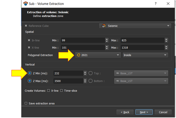
1. To draw a polygon, the easiest way is to open the seismic survey or a horizon map view (horizon stack or single horizon if you already had) or a Timeslice viewer (might take a while to generate) so it is recommended to use survey or horizon viewer.
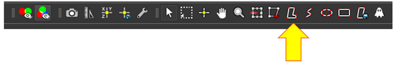
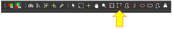
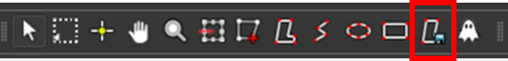
2. Go to the main toolbar, select the Closed Polygon option.
3. Left click on the viewer to drop a point and create the shape of the polygon, then double click to close the polygon.
You can edit the anchor points by click on the Anchor Point Edition icon and double click on the polygon to move its anchor points to get the best shape of the polygon as well.
 on the main toolbar to save it.
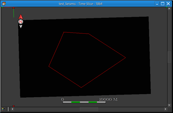
5. You can then save it in different formats (if you want to export it later in shapefile format, select the culture option, otherwise just Polyline option is enough), put a name for it and hit ok.
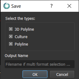
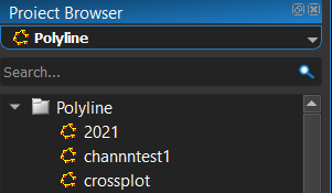
The polyline will be saved in the Polyline folder of the Project Browser and will appear on the list on the Volume Extraction interface - Polygon list to use for the extraction.
The vertical window size represents the number of samples taken into account for the calculation of the attribute, centred on the horizon. For instance, if the user takes a vertical window size of 7 samples, this means PaleoScan will take into account 3 samples above the horizon, 1 sample along the horizon and 3 samples below the horizon. The size of one sample corresponds to the vertical resolution of the volume.
The type of input volumes on which the different attributes can be calculated can be identified thanks to the icons.
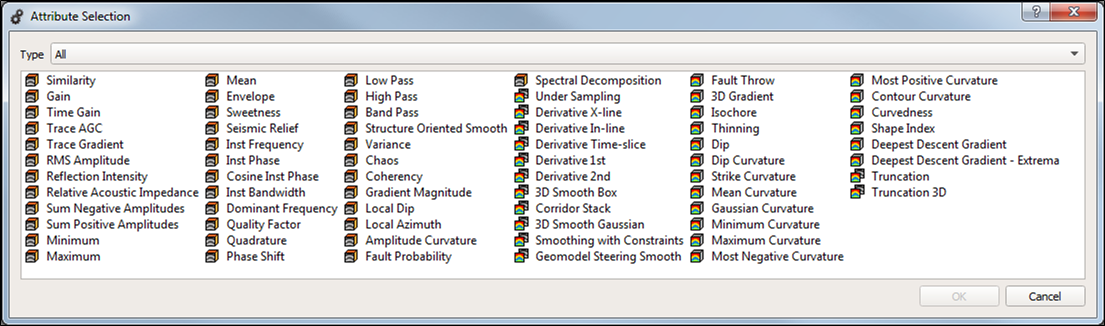
 Attribute to be computed on seismic volumes
 Attribute to be computed on Geomodel
 Attribute to be computed on seismic volumes and/or Geomodels
Real-time attributes are calculated along the plan of the displayed section, therefore, only 2D attributes can be generated. An attribute based on 3D computations would be too computationally expensive to display that way.
2D Lines & 2D Workflows
For the time being, you must crop each 2D Line of a set at a time by according to the extent you expect of it.
To do so, you should follow these steps:
1. From the 2D Line toolbar, click on the '2D Line Conditioning' tool,
2. Drag and drop all the 2D Lines that need to be cropped in the left panel of the displayed interface,
3. Select one single 2D Line from the list,
4. Check on the ‘Vertical’ and 'Spatial' cropping mode,
5. Enter the number of splits (crops spatial boundaries) that your need,
6. Activate the Slider button to adjust the position of the cropping boundaries vertically and laterally,
7. Click on Save.
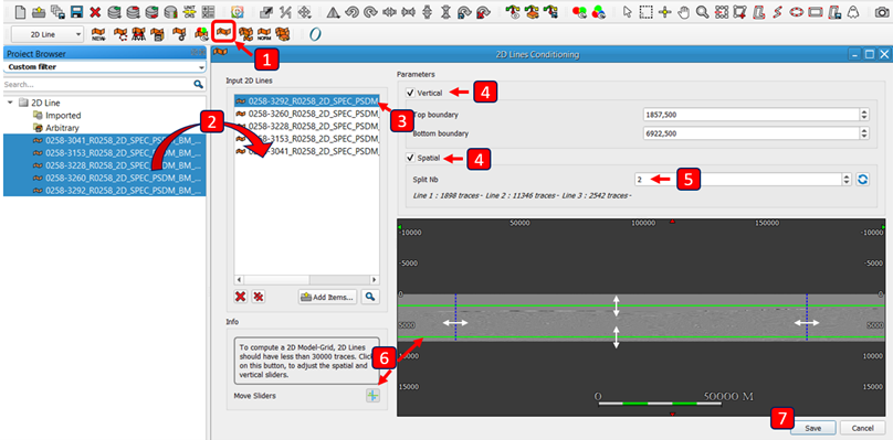
8. Repeat 2 through 6 for as many 2D Lines as necessary.
9. Gather all the pieces of output cropped lines to create a 2D Line Set (that should match the desired cropping extent).
The shapefile you imported is considered in PaleoScan as a Culture Data. You will not be able to use this ‘Culture’ Data as input to create the arbitrary line because it only considers ‘Polyline’ objects.
As a workaround, you can follow this workflow:
Convert your Culture Data into a Polyline
1- Open the culture data .
2- Double click on it to select it (F mouse mode).
3- Click on the Save Polyline icon

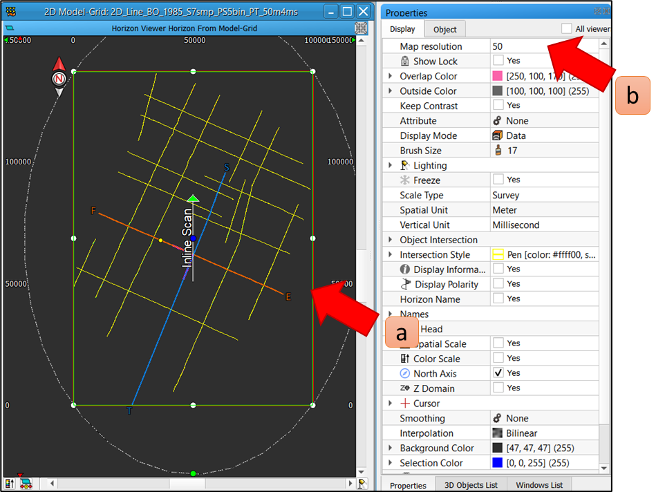
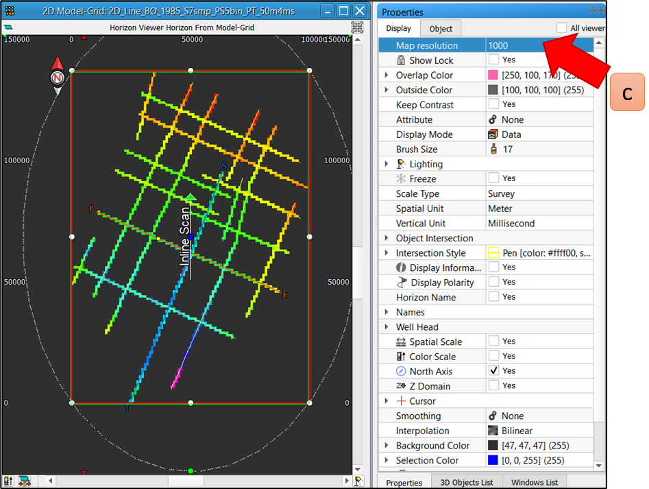
You can change the Horizon Viewer resolution, and this will show the 2D horizon thicker than the yellow lines:
a) You will have to select (using the selection mouse mode F) the green box surrounding the line set in the Horizon viewer
b) In the Properties/Display, you will see the first option for "Map resolution":
You can of course create arbitrary line in PaleoScan. For that purpose, select the 2D Line module toolbar.

Then, there are two options to create an arbitrary line:
Option 1: The first option aims at creating an arbitrary line based on the positions of wells.
- Click on the third button starting from the left
 New Arbitrary Line Along Wells. In this application, you will first need to drag and drop the wells you wish to use to define the path of the arbitrary line.
 - Drag and drop the volume to extract along this line.
- Once done, click on the following button Search Optimum Trajectory located in the middle of the application. PaleoScan will this way find the best trajectory along the selected wells.
- Finally, if you wish to save the arbitrary line, define an output name and click on OK.
Option 2: The second option aims at creating an arbitrary line based on a random polyline.
- Open a seismic line and display it as a time slice using the Volume Manager.
- Click on the first button of the 2D Line toolbar New > Arbitrary Line Creation.
- Now you will have a specific mouse mode that allows you to pick the trajectory of the arbitrary line in the time slice viewer. Double click for ending the picking of the trajectory.
- An application should pop up.
- Select the volume to extract along the line and click on next. If you wish to save the line you will need to define an output name and click on OK. If you already have an arbitrary line in your project, you can display it in a map, select it and click on the second button of the 2D Line toolbar New Arbitrary Line from Polyline. You will skip the 3 first points of this workflow. The following steps are the same.
For both options, the arbitrary line saved will be stored under the 2D Line tab of the Project Browser.
Yes, the 3D automatic horizon tracking workflow can also be applied to 2D lines. 3D Geo-Models and Horizon Stacks can be generated from 2D lines interpretation.
In PaleoScan, the mis-tie corrections applied to 2D line is not static but variant, it is therefore not possible to define a specific 2D line as a reference for the correction. All the 2D lines move up or down in relation to one another, according to the marked horizons.
2D lines can be added to an existing 2D Model-Grid by right clicking on an existing 2D interpretation and selecting the Add 2D Line(s) option from the pull-down menu. This option is also available from the Model-Grid toolbar. The user will then need to run an Automatic Propagation in order to generate links between nodes on the added 2D lines.

On 2D Model-Grids, the Geo-Model preview is computed and displayed according to the marked horizons only. Therefore, the user first needs to mark at least two horizons before launching the preview.
Yes, it is possible. To do so the user needs to have generated a 2D Horizon Stack. They then need to use the 2D Horizon Stack Interpolation option to generate a 3D Horizon Stack. This option is available from the Horizon Stack toolbar, from the Project Browser context menu or from the 2D Horizon Stack context menu.

Finally, the 3D Geo-Model from Horizons tool, available from the Horizon toolbar can be used to generate the 3D Geo-Model, using the 2D interpolated Horizon Stack as an input.

Workflows
As you already have a polyline, please do a right click on the horizon you want to use and select the option called "Extract". Then select the polyline, click on next, give a name and click on finish.
We end up with just a part of the horizon based on the polyline:
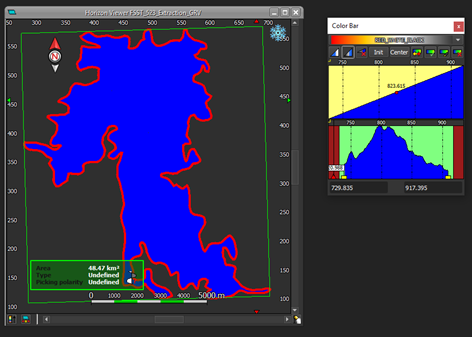
Now that we have our horizon, we can perform the GRV workflow.
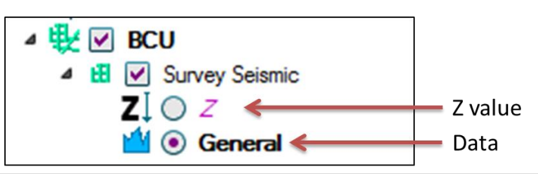
From the Properties tab, set the display mode (2nd option) to "Z-value":
Select the entire horizon by making it blue (from the color bar widget):
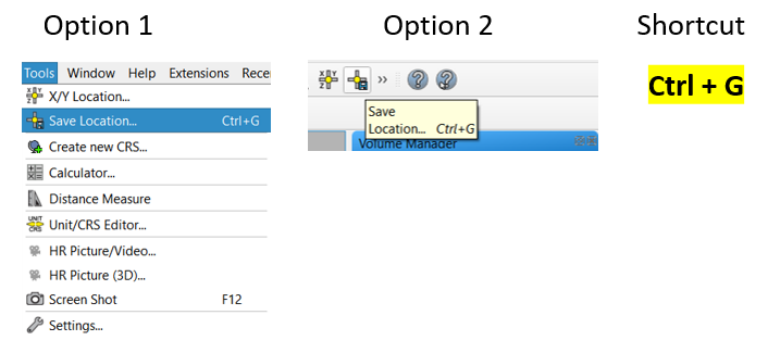
There is a useful tool in PaleoScan to save a location to return to it at a later stage.
To save any location, first you will have to position the cursor (the cross-navigation mode) on the exact place you want to keep. Then, click on the Save Location option under the main tool bar (or press CTRL + G).
An box opens, asking you to give a name to the location. You may also add a description by ticking the “Add description” checkbox.
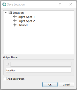
In the end, you can find all your saved locations in your Project Browser, under the Location label in the Polyline tab.

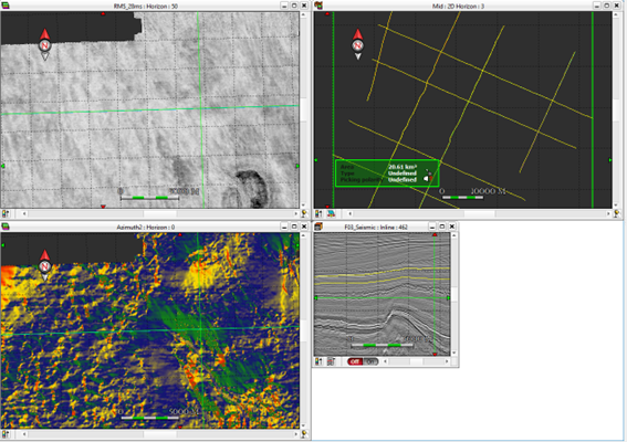
You can't tile specific windows, but there's a slightly hidden workaround to do it from the "Windows List".
Let's say you open 4 windows and want to have just 1 minimized (with all the others at the same scale).
From the "Windows List", select the one you want to custom and click on the 4th button "Resize / Synchronize size".
You can then specify a "Custom size" on how big you want your window to be.
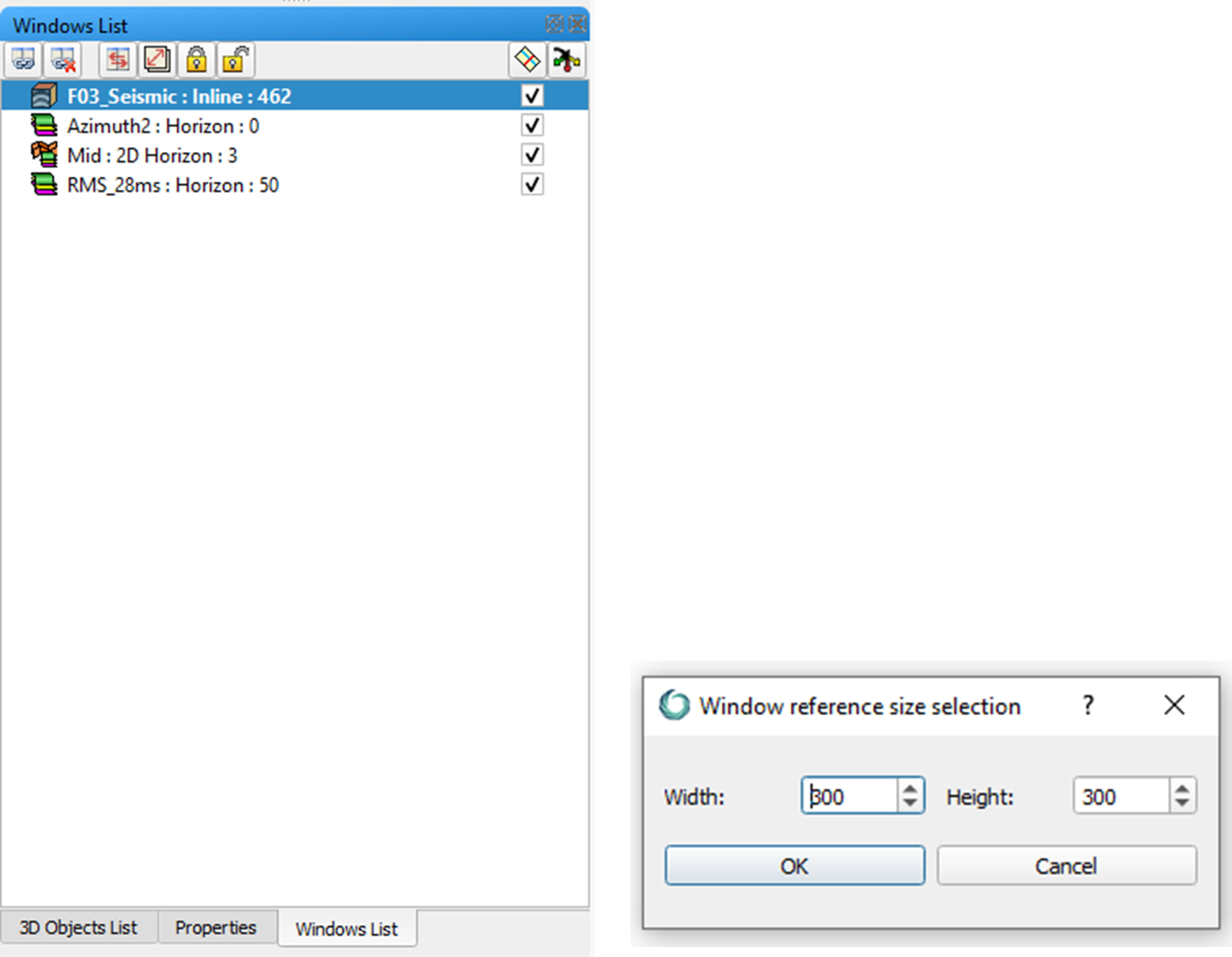
And finally, you can tile your windows afterward.
You can change them all at once or individually. In the example below, we used a custom size of 300 x 300 for the "F03_Seismic".
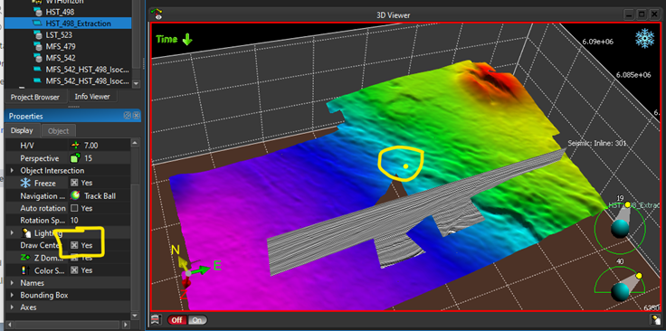
The "Draw Center" check box refers to the yellow dot which is what we call the "Focal Point". You can set this as the center of rotation by double-clicking on an object in the 3D window with the "Cross-Navigation" mouse mode enabled.
You might notice that when you use the "Cross-Navigation" mode in a 2D window there will be a yellow dot following your cursor around. This is the same object you see in the 3D window.
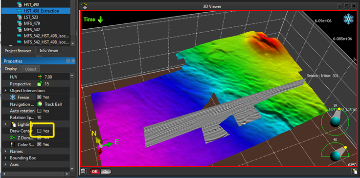
To remove the yellow dot in the 3D window first double-click in the black background of the 3D window to select it.
Next, go to your properties pane and unselect the "Draw Center" option as seen below...
Yellow dot "on"...
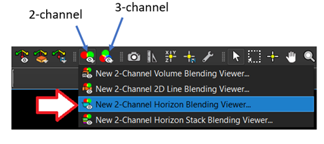
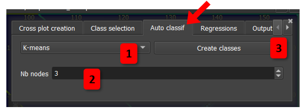
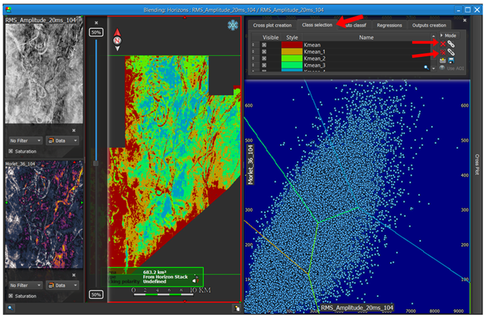
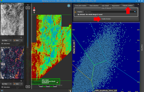
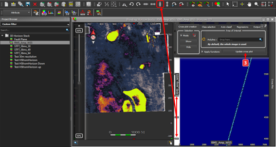
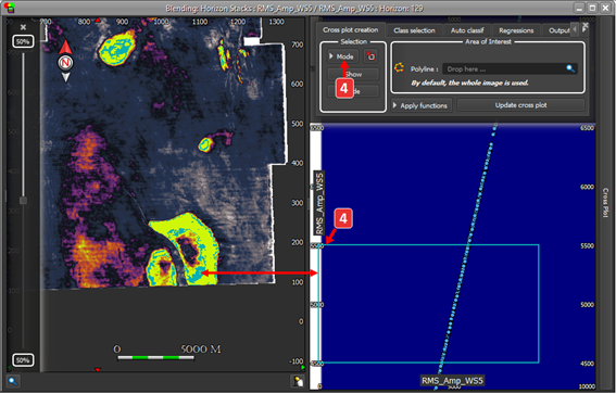
In PaleoScan, you can use 2-channel or 3-channel cross plot on a single horizon with different attributes and then classify the facies using the SOM or K-mean.
Here is the workflow:
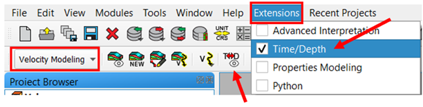
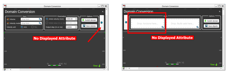
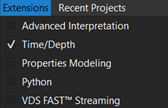
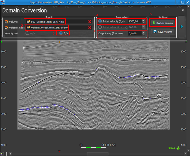
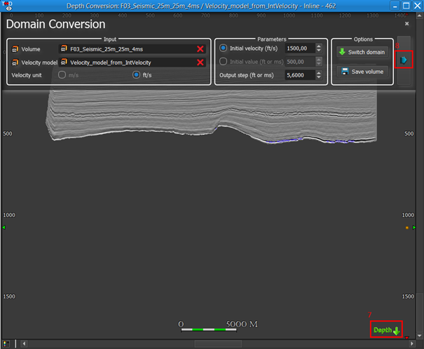
First, you will probably have to activate the Time/Depth extension. Then, go in the Velocity Modeling module and click on the Domain Conversion tool:
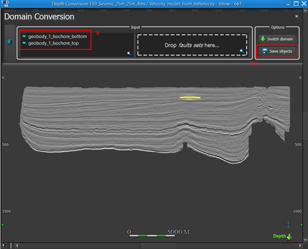
To convert objects in addition to the volume, you have to click on the blue arrow. Then you will see the place where to drop the horizons you want to convert:
If you want to convert a horizon stack, you will have to do a little trick, as in the Domain conversion window you can only drop individual horizons.
The first thing to do will be to extract all the horizons from your horizon stack (i.e., create each horizon individually).
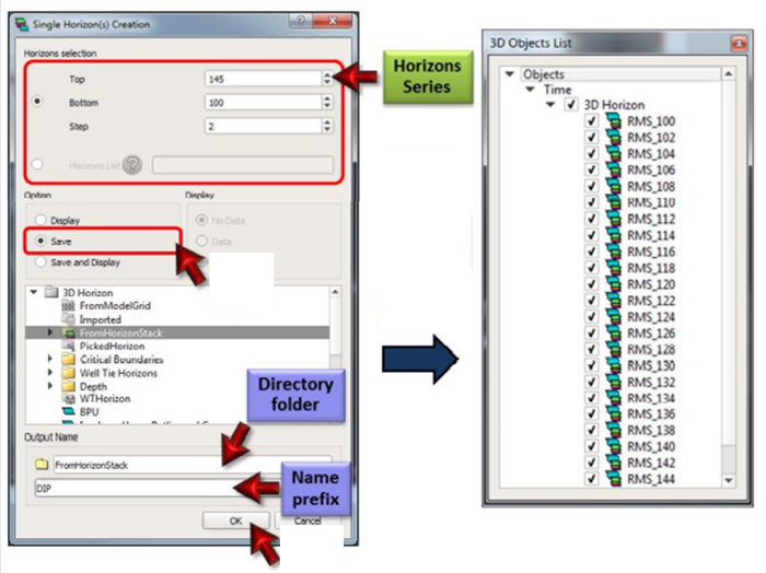
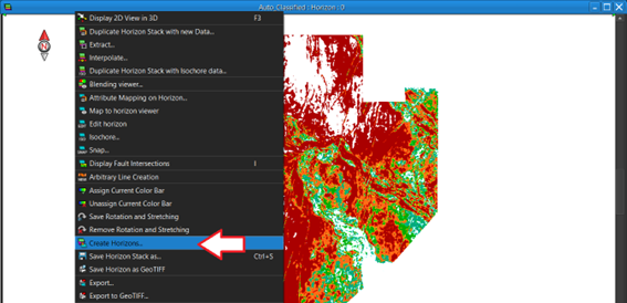
To do so, open you horizon stack, right click on the top bar, select "Create Horizons”, and define the options:
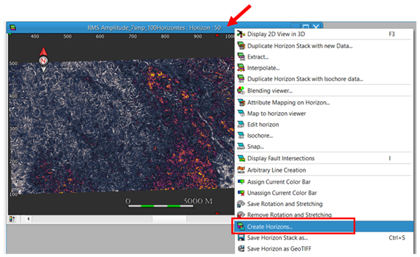
On the top bar of the horizon stack, you have the number of the displayed horizon. When you open a Horizon stack, it automatically displays the horizon at the middle of the stack. In this case, we had created a horizon stack with 100 horizons, so what we are seeing is the number 50. When you want to create single horizons, you can change the number of the bottom and top horizon. In the example below, I wanted to extract all the horizons, so I put horizon 0 for the bottom and 99 for the top. But you could also extract the horizons with a step of 2, or more. You can also define a horizon list, the same way we do with a printer. You can let the same name; every created horizon will have this name + its number. Click on OK:
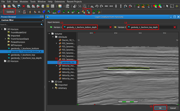
It is necessary to generate top and bottom horizons, convert them in depth with the velocity model, and generate a depth converted layer from them.
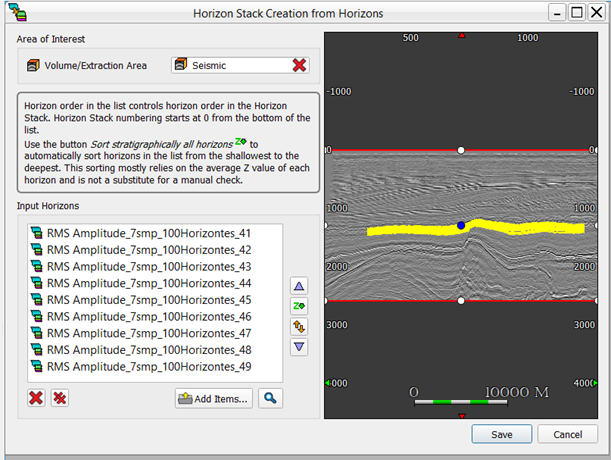
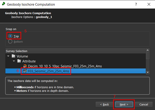
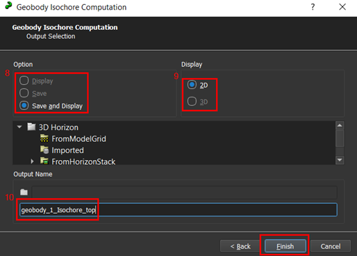
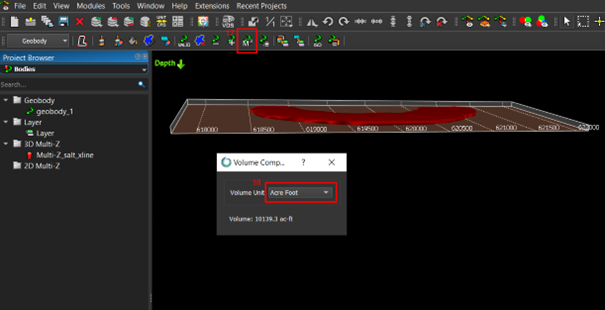
In the Geobody module (1 in the figure below), with the Geobody Isochore Computation tool (2), select the Geobody of interest (3) and click on Next (4).
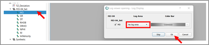
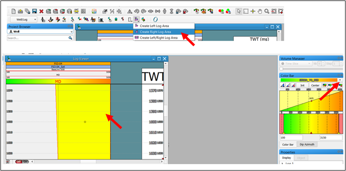
To create a log template, please, follow the following steps:
1- Open a log
- Double-click on one of your log from the Project Browser, set No log area and click Ok
- Open the Well/Log module
- Select your log (double click on the log)
- Click on Log Area Management and select Create Right Log Area (or one of the options)
- Then, double click inside the log to select it and change the color bar on the right-hand side.
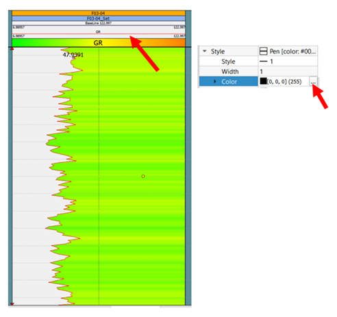
- You can also change the color of the log curve, by double-clicking on the line below GR (see the red arrow) and going into Properties - Display tab (right-hand side of your screen).
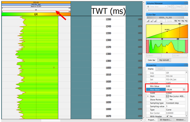
- If you double-click again in the same place, you can also change the Min and Max values of the log.
- Double-click on the track to select it,
- Hit the Save selected object icon. Give it a name and press Ok.
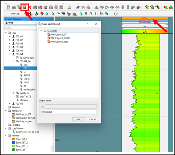
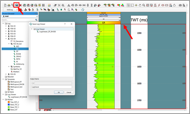
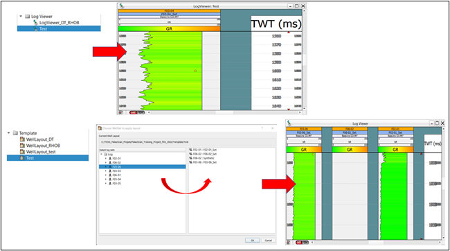
- The log viewer corresponds to the opened logs when you save it
- The Template allows you to display several logs in the same viewer with same set and style.
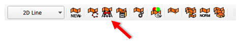
There is a simple way to create an arbitrary line along wells in PaleoScan.
To generate this line:
Click on “New Arbitrary Line Along Wells”
1. Drag and drop the required wells from the project browser in the Well list.
2. Sort the wells in the list to adjust the polyline, by moving them up or down (the polyline is computed and displayed in real time on a map according to the wells sorting). The interface offers the possibility to automatically sort the wells to get the most optimized trajectory. To do so, press the “Search optimum trajectory” button (2a).
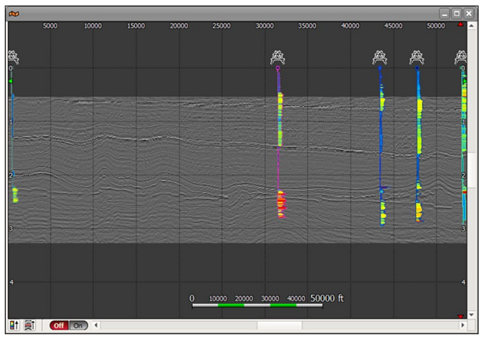
3. Drag and drop the reference volume used to map the information on the Arbitrary Line.
4. Define the extension of the Arbitrary Line around its edges. The direction of the extension is guided by the deviation of the well.
5. Select the option Display or Save and Display. If the Save option is enabled, enter the name of the Arbitrary Line.
6. Click on “Ok” to create the Arbitrary Line.
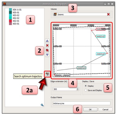
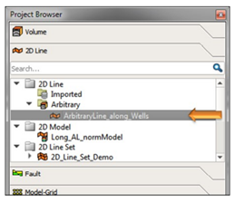
Finally, the arbitrary line along the wells is saved & stored in the 2D Line tab of the project browser under the name "Abritrary_line_along_wells".
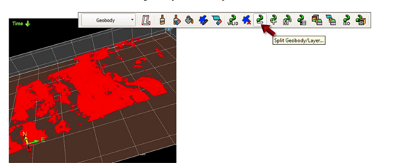
In PaleoScan, there are only workflows to split a geobody: the "Split Geobody/Layer" option & the "Crossplot".
- Option 1:
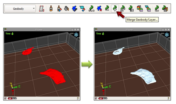
The first workflow is to try splitting the geobody into small geobodies (disconnected pieces). Then, you can choose which one you would like to activate/display in the 3D viewer. You can later choose to merge them into a unique geobody.
In the 3D viewer, select the Layer/Geobody to be split by double-clicking on it with the selection mouse mode. Then click on the Split Layer/Geobody button in the toolbar.
- Option 2:

1. Import data into PaleoScan: seismic, faults, wells, markers, culture data.
2. Insert or interpret constraint areas in PaleoScan: faults, salt (Multi-Z).
3. Model-Grid computation:
- Choose the right Model-Grid parameters for the seismic: patch size, polarity, smooth level, undersampling.
- Refine the AutoInterp Model-Grid (horizon editing), using the cross-navigation mouse mode (G shortcut) and then W to activate horizons and M to mark them.
- Quality check the interpretation using preview modes.
4. 3D Geo-Model Computation:
- Choose the 3D Geo-Model parameters: smooth size, link probability, interpolation size.
- Quality check the Geo-Model.
5. 3D Geo-Model applications:
- Basic platform: Horizon Stack, Attributes, Geobody modelling, Fault management, Salt management, Well correlation.
- Add-on modules: Sequence stratigraphy, Automatic geobody extraction, Property modelling, RGB blending, Well tie, Coloured inversion, Spectral blueing.
1. Disconnect Patches of Active Horizon: to disconnect all the patches composing the active horizon displayed in the Horizon Viewer, the user needs to click on the Disconnect All Patches From Active Horizon button in the Model-Grid toolbar. The current horizon will progressively disappear from the Horizon Viewer. This horizon will no longer be taken into account in the Model-Grid interpretation, it can then be picked again in a better way.


1. Click on the Spectral Decomposition tool in the Attributes toolbar

2. Drag and drop the input volume into the Volume selection area.
Then, use the cross-navigation mouse mode to select a trace that shows an event of interest. The frequency spectrogram along the seismic trace will be displayed. The method to use, either Short Time Fourier Transform or Continuous Wavelet Transform, and its corresponding parameters can be chosen.

3. Using the Frequency Picking mouse mode, double click on the Spectrogram viewer to select frequencies. The selection of the frequency can be laterally adjusted and a preview of the current selected frequency decomposition is then displayed:

4. Save the outputs: create volumes or real-time attributes.
If three frequencies have been selected and the Advanced Interpretation add-on module is activated, the three resulting real-time attributes from this interface can be sent to a volume colour blending viewer, using the Send to RGB Viewer button.
5. Display the results on Horizon Stacks
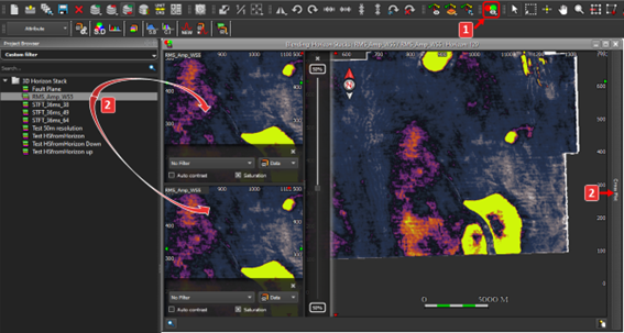
Open a Horizon Stack, right click on the window and select Duplicate Horizon Stack with new attribute or create a new one. Then, select the None filter and drag and drop the saved volume or real-time attribute from Spectral Decomposition. Several Horizon Stacks can be created at the same time by clicking on the cross at the top of the window, especially if several volumes with different frequencies have been computed. Then click on Run to create the Horizon Stacks.

If the frequencies and parameters to be applied are already known, Spectral Decomposition can be selected as the filter option. The Horizon Stack can then be directly created without computing new volumes or real-time attributes.

Once the 3 Horizon Stacks have been created, they can be displayed in a Horizon Stack Color Blending Viewer to help the seismic interpretation (if the Advanced Interpretation add-on module is activated). This tool is available from the Color Blending toolbar. The colour blending can also be displayed in the 3D viewer.
1. Create a 2D line set with the desired 2D lines using the New 2D Line Set button available from the 2D Line toolbar:

2. Generate a 2D Model-Grid on the 2D line set that has been created. Click on the New 2D Model-Grid button available from the Model-Grid toolbar and select the desired 2D line set as input

3. Refine the Model-Grid using the same tools as for a 3D Model-Grid (Cross-navigation mouse mode, W shortcut to activate a horizon, M to mark it)

4. Generate the 2D Geo-Model using the Compute Geo-Model button available from the Model-Grid toolbar
5. Generate a 2D Horizon Stack using the New 2D Horizon Stack button of the Horizon Stack toolbar


