Icon décoration

PaleoScan™ Geobody Extraction

PaleoScan™ Geobody Extraction

3D Geobody extraction is a fundamental aspect of seismic interpretation as geobodies can represent geological features which may impact reservoir prediction and characterization.

PaleoScan™ 2018 includes innovative workflows to enhance the imaging and extraction of geological features from seismic data with greater efficiency and accuracy in comparison with conventional techniques.

The 3D Relative Geological Time (RGT) model and the Horizon Stack are unique products from PaleoScan™ which allow the user to use an unlimited number of chronostratigraphic surfaces for stratigraphic analysis.

In PaleoScan™ a wide variety of seismic attributes can be calculated on a 3D seismic volume and the Horizon Stack. These can be used to help the user in identifying and extracting geological features in an accurate way in terms of both the RGT stratigraphy and seismic expression. PaleoScan™ offers integrated tools to directly map and extract geobodies from a seismic volume and a Horizon Stack.
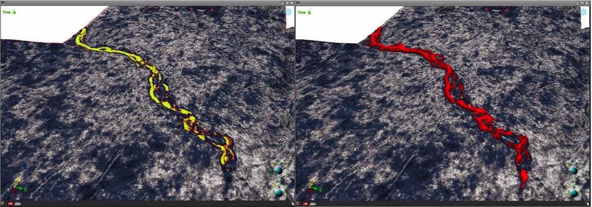
1. Brush tool

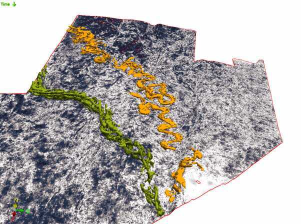
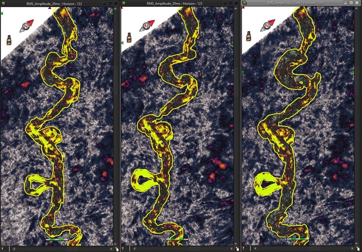
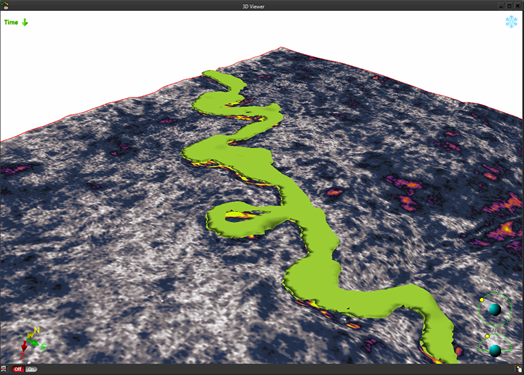
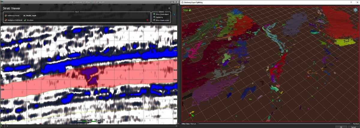
The user can manually map a geobody in PaleoScan™ by simply brushing over the geological features on each horizon of the Horizon Stack where the geobody can be recognized (Fig. 1). By this method, the geobody is delineated and modified interactively throughout the Horizon Stack. When the geobody delineation is finished PaleoScan™ will validate the Geobody by interpolating between those mapped polygons in the Horizon Stack (Fig. 2).
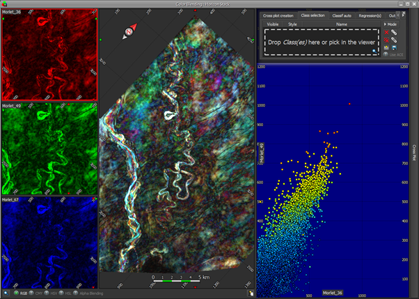
Figure 1: Channel-belt feature is delineated on horizons in the Horizon Stack using the Brush mode, Each horizon is 3-5 ms apart, and the geobody is interpolated from each of these polygons.
Figure 2: Geobody is built by interpolating between mapped polygons on these above horizons.

2. Colour Bar mode

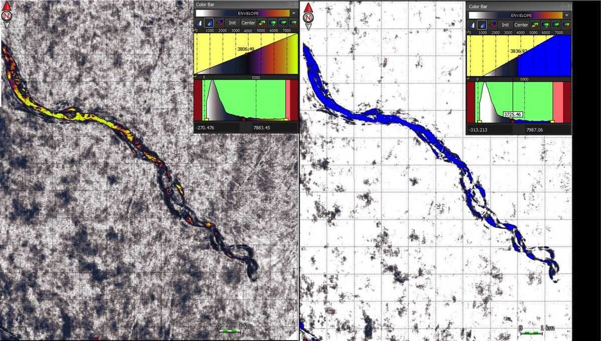
Still working on the Horizon Stack, the user can isolate values of a mapped attribute by manipulating the colour bar (Fig. 3) and then extracting and saving these values as an independent object in PaleoScan™ (Fig. 4).

Figure 3: (Left) Channel-belt feature on RMS attribute horizon and its original Colour Bar (Right) New Colour Bar is applied on RMS attribute horizon to isolate the channel-belt feature.
Figure 4: (Left) Channel-belt feature on RMS attribute horizon in 3D domain. (Right) Channel-belt geobody is saved and then displayed in 3D domain as a result of amplitude extraction using Colour Bar mode.

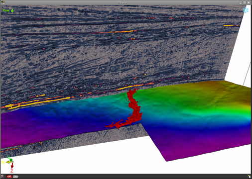
3. Geobodies from 3D Volume

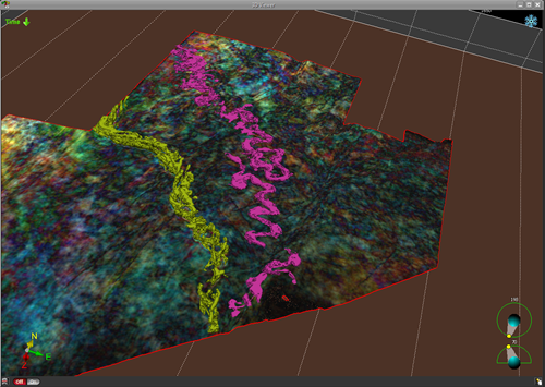
Thanks to the Sequence Stratigraphy module in PaleoScan™, geobodies representing channels, salt domes, volcanics and clinoforms (among others) can be constrained and picked directly from the 3D seismic volume. The extractions are within the 3D sequence stratigraphic framework and filtered by Geobody Filter tool to have the best result.

Figure 5: (left) Amplitude associated with the channel-belt feature is isolated by Colour Bar mode and constrained within the red sequence from Strati Viewer. (right) Channel-belt and unrelated geobodies are extracted and filtered in the Geobody Filter tool in PaleoScan™.
Figure 6: Channel-belt geobodies after filtering are displayed in 3D viewer.

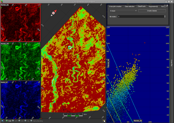
4. Using Machine Learning for Geobody extraction

PaleoScan™ offers two Machine Learning methods to automatically define classes/facies on a crossplot. Geobodies for each class/facies are generated automatically within the whole volume or a specific interval.

Figure 7: (above) Using Spectral Decomposition seismic attribute and the Colour Blending tool to hightlight the geological features and their values on the crossplot. (below) PaleoScan™ categorizes the crossplot values into 5 main classes using clustering algorithms (K-mean, Self-organising Map).
Figure 8: Channel-belt geobodies created from an automatically classified crossplot are displayed in the 3D viewer.

Volumetrics:

Once the Geobodies have been validated, a fast volumetric calculation can be calculated for each Geobody. If the Geobody delineation is in the time domain, a time-depth relationship must be applied to compute the volume of the geobody.

To find out more about the Geobody extraction, drop us a line at contact@eliis.fr

Case study: Maui 3D, Taranaki Basin, New Zealand. RMS amplitude seismic attribute. Spectral Decomposition seismic attribute.

Drop us a line !

Stay connected !

Stay connected !